THE FRACTAL STRUCTURE OF DATA REFERENCE- P18 docx
Bạn đang xem bản rút gọn của tài liệu. Xem và tải ngay bản đầy đủ của tài liệu tại đây (97.97 KB, 5 trang )
Free Space Collection in a Log 73
must be moved (i.e. read from one location and written back to another). For
storage utilizations higher than 75 percent, the number of moves per write
increases rapidly, and becomes unbounded as the utilization approaches 100
percent.
The most important implication of (6.1) is that the utilization of storage
should not be pushed much above the range of 80 to 85 percent full, less any
storage that must be set aside as a free space buffer. To put this in perspective,
it should be noted that traditional disk subsystems must also be managed so
as to provide substantial amounts of free storage.
Otherwise, it would not
be practical to allocate new files, and increase the size of old ones, on an as
-
needed basis. The amount of free space needed to ensure moderate freespace
collection loads tends to be no more than that set aside in the case of traditional
disk storage management [32].
The final two sections of the chapter show, in a nutshell, that (6.1) continues
to stand up as a reasonable “rule of thumb”, even after accounting for a much
more realistic model of the free space collection process than that initially
presented to justify the equation. This is because, to improve the realism of the
model, we we must take into account two effects:
1. the impact of transient patterns of data reference within the workload, and
2. the impact of algorithm improvements geared toward the presence of such
patterns.
Figure 6.1.
Overview of free space collection results.
74
One section is devoted to each of these effects. As we shall show, effects (1)
and (2) work in opposite directions, insofar as their impact on the key metric
M is concerned. A reasonable objective, for the algorithm improvements of
(2), is to ensure a level of free space collection efficiency at least as good as
that stated by (6.1).
Figure 6.1 illustrates impacts (1) and (2), and provides, in effect, a road map
for the chapter. The heavy solid curve (labeled linear model), presents the
“rule
-
of
-
thumb” result stated by (6.1). The light solid curve (labeled transient
updates), presents impact (1). The three dashed lines (labeled tuned / slow
destage, tuned / moderate destage, and tuned / fast destage) present three cases
of impact (2), which are distinguished from each other by how rapidly writes
performed at the application level are written to the disk medium.
1.
In a log
-
structured disk subsystem, the “log” is not contiguous. Succeeding
log entries are written into the next available storage, wherever it is located.
Obviously, however, it would be impractical to allocate and write the log one
byte at a time. To ensure reasonable efficiency, it is necessary to divide the log
into physically contiguous segments. A segment, then, is the unit into which
writes to the log are grouped, and is the smallest usable area of free space. By
contrast with the sizes of data items, which may vary, the size of a segment is
fixed. The disk storage in a segment is physically contiguous, and may also
conform to additional requirements in terms of physical layout.
A segment may contain various amounts of data, depending upon the detailed
design of the disk subsystem. For reasons of efficiency in performing writes,
however, a segment can be expected to contain a fairly large number of logical
data items such as track images.
Let us consider the “life cycle” of a given data item, as it would evolve along
a time line. The time line begins, at time 0, when the item is written by a host
application.
Before the item is written to physical disk storage, it may be buffered. This
may occur either in the host processor (a DB2 deferred write, for example) or
in the storage control. Let the time at which the data item finally is written to
physical disk be called τ
0
.
As part of the operation of writing the data item to disk, it is packaged into
a segment, along with other items. The situation is analogous to a new college
student being assigned to a freshman dormitory. Initially, the dormitory is full;
but over time, students drop out and rooms become vacant.
In the case of a
log structured disk subsystem, more and more data items in an initially full
segment are gradually rendered out
-
of
-
date.
Free space collection of segments is necessary because, as data items con
-
tained in them are superseded, unused storage builds up. To recycle the unused
THE FRACTAL STRUCTURE OF DATA REFERENCE
THE LIFE CYCLE OF LOGGED DATA
Free Space Collection in a Log 75
storage, the data that are still valid must be copied out so that the segment
becomes available for re
-
use — just as, at the end of the year, all the freshmen
who are still left move out to make room for next year’s class.
In the above analogy, we can imagine setting aside different dormitories
for different ages of students — e.g., for freshmen, sophomores, juniors and
seniors. In the case of dormitories, this might be for social interaction or mutual
aid in studying. There are also advantages to adopting a similar strategy in a log
-
structured disk subsystem. Such a strategy creates the option of administering
various segments differently, depending upon the age of the data contained in
them.
To simplify the present analysis as much as possible, we shall assume that
the analogy sketched above is an exact one. Just as there might be a separate
set of dormitories for each year of the student population, we shall assume that
there is one set of segments for storing brand new data; another set of segments
for storing data that have been copied exactly once; another for data copied
twice; and so forth.
Moreover, since a given segment contains a large number of data items,
segments containing data of a given age should take approximately the same
length of time to incur any given number of invalidations. For this reason, we
shall assume that segments used to store data that have been copied exactly
once consistently retain such data for about the same amount of time before it
is collected, and similarly for segments used to store data that have been copied
exactly twice, exactly three times, and so forth.
To describe how this looks from the viewpoint of a given data item, it
is helpful to talk in terms of generations. Initially, a data item belongs to
generation 1 and has never been copied. If it lasts long enough, the data item is
copied and thereby enters generation 2; is copied again and enters generation
3; and so forth. We shall use the constants τ
1
, τ
2
, , to represent the times
(as measured along each data item’s own time line) of the move operations just
described. That is, τ
i
, i = 1, 2, . . ., represents the age of a given data item
when it is copied out of generation i.
2. FIRST
-
CUT PERFORMANCE ESTIMATE
Let us now consider the amount of data movement that we should expect to
occur, within the storage management framework just described.
If all of the data items in a segment are updated at the same time, then
the affected segment does not require free space collection, since no valid
data remains to copy out of it. An environment with mainly sequential files
should tend to operate in this way. The performance implications of free
space collection in a predominately sequential environment should therefore
be minimal.
76
THE FRACTAL STRUCTURE OF DATA REFERENCE
In the remainder of this chapter, we focus on the more scattered update
patterns typical of a database environment. To assess the impact of free space
collection in such an environment, two key parameters must be examined: the
moves per write M, and the utilization of storage
u. Both parameters are
driven by how empty a segment is allowed to become before it is collected.
Let us assume that segments are collected, in generation i , when their storage
utilization falls to the threshold value f
i
.
A key further decision which we must now make is whether the value of the
threshold f
i
should depend upon the generation of data stored in the segment. If
f
1
= f
2
= . . = f, then the collection policy is history independent since the
age of data is ignored in deciding which segments to collect. It may, however, be
advantageous to design a history dependent collection policy in which different
thresholds are applied to different generations of data. The possibilities offered
by adopting a history dependent collection policy are examined further in the
final section of the chapter. In the present section, we shall treat the collection
threshold as being the same for all generations.
Given, then, a fixed collection threshold f, consider first its effect on the
moves per write M. The fraction of data items in any generation that survive to
the following generation is given by f, since this is the fraction of data items
that are moved when collecting the segment. Therefore, we can enumerate the
following possible outcomes for the life cycle of a given data item:
The item is never moved before being invalidated (probability 1 – f).
The item is moved exactly once before being invalidated (probability f x
(1 – f )).
The item is moved exactly i = 2, 3, . . . times before being invalidated
(probability f
i
x (1 – f)).
These probabilities show that the number of times that a given item is moved
conform to a well
-
known probability distribution, i.e. the
geometric
distribution
with parameter f. The average number of moves per write, then, is given by
the average value of the geometric distribution:
(6.2)
Note that the moves per write become unbounded as f approaches unity.
Next, we must examine the effect of the free space collection policy on
the subsystem storage utilization u. Intuitively, it is clear that to achieve high
storage utilization, a high value of f will be required so as to minimize the
amount of unused storage that can remain uncollected in a segment.
There is a specific characteristic of the pattern of update activity which, if
it applies, simplifies the analysis enormously. This characteristic involves the
Free Space Collection in a Log
77
average utilization experienced by a given segment over its lifetime (the period
between when the segment is first written to disk and when it is collected). If
this average utilization depends upon the collection threshold f in the same
way, regardless of the generation of the data in the segment, then we shall
say that the workload possesses a homogeneous pattern of updates. Both the
simple model of updates that we shall assume in the present section, as well
as the hierarchical reuse model examined in the following section, exhibit
homogeneous updates.
If the pattern of updates is homogeneous, then all segments that are collected
based on a given threshold will have the same average utilization over their
lifetimes. In the case of a single collection threshold for all segments, a single
lifetime utilization must also apply. This utilization must therefore also be the
average utilization of the subsystem as a whole, assuming that all segments are
active.
Let us now make what is undoubtedly the simplest possible assumption about
the pattern of updates during the life of a segment: that the rate of rendering
data objects invalid is a constant. In the dormitory analogy, this assumption
would say that students drop out at the same rate throughout the school year.
We shall call this assumption the linear model of free space collection.
By the linear model, the utilization of a given segment must decline, at
a constant rate, from unity down to the value of the collection threshold.
Therefore the average storage utilization over the life of the segment is just:
(6.3)
Since this result does not depend upon generation, the linear model has a
homogeneous pattern of updates. Equation (6.3) gives the average lifetime
utilization for any segment, regardless of generation. Therefore, (6.3) also
gives the utilization of the subsystem as a whole, assuming that all segments
are active (i.e., assuming that no free space is held in reserve). As expected,
storage utilization increases with f .
We need now merely use (6.3) to substitute for f in (6.2). This yields the
result previously stated as (6.1):
This result is shown as the heavy solid curve in Figure 6.1. It shows clearly that
as the subsystem approaches 100 percent full, the free space collection load
becomes unbounded. This conclusion continues to stand up as we refine our
results to obtain the remaining curves presented in the figure.
It should be noted that, due to our assumption that all segments are active,
(6.1) applies only to storage utilizations of at least 50 percent. For lower