THE FRACTAL STRUCTURE OF DATA REFERENCE- P26 doc
Bạn đang xem bản rút gọn của tài liệu. Xem và tải ngay bản đầy đủ của tài liệu tại đây (118.35 KB, 5 trang )
Disk Applications: A Statistical View
115
The initial two sections of the chapter introduce the basic structure of the
deployable applications model, and examine the calculation of application
characteristics. The final two sections then turn to the implications of the model
with respect to disk performance requirements, seeking a common ground
between the two contrasting views outlined at the beginning of the chapter.
1. DEPLOYABLE APPLICATIONS MODEL
Consider an application a, with the following requirements:
v
a
= transaction volume (transactions per second).
s
a
= storage (gigabytes).
The purpose of the deployable applications model is to estimate whether
such an application will be worthwhile to deploy at any given time. Thus, we
must consider both the benefit of deploying the application, as well as its costs.
Application a will be considered deployable, if its costs are no larger than its
estimated benefits.
The benefit of application a is tied to desired events in the real world, such as
queries being answered, purchases being approved, or orders being taken. Such
real
-
world events typically correspond to database transactions. Therefore, we
estimate the dollar benefit of application a from its transaction volume:
(9.1)
where k
1
is a constant.
For the sake of simplicity, we divide application costs into just two categories.
Transaction processing costs, including
CPU costs and hardware such as point
-
of
-
sale terminals or network bandwidth upgrades, are accounted for based upon
transaction volume:
(9.2)
where k
2 ≤
k
1
.
To account for the storage costs of application a, we examine the resources
needed to meet both its storage and
I/O requirements. Its storage requirements
have already been stated as equal to s
a
. In keeping with the transaction
-
based
scheme of (9.1) and (9.2), we characterize application a’s
I/O requirement (in
I/O’s per second) as Gv
a
, where G is a constant (for simple transactions, G
tends to be in the area of 10
-
20 I/O’s per transaction).
Against the requirements of the application, as just stated, we must set
the capabilities of a given disk technology. Let the disk characteristics be
represented as follows:
p = price per physical disk, including packaging and controller functions
(dollars).
116
c = disk capacity (gigabytes).
y = disk throughput capability (
I/O’s per second per disk).
x = y/G = disk transaction
-
handling capability (transactions per second per
D = average disk service time per
I/O (seconds).
To avoid excessive subscripting, the specific disk technology is not identified in
the notation of these variables; instead, we shall distinguishbetween alternative
disk technologies using primes (for example, two alternative disks might have
capacities c and c').
Based on its storage requirements, we must configure a minimum of s
a
/c
disks for application a; and based on its transaction
-
processing requirements,
we must configure a minimum of v
a
/x disks. Therefore,
THE FRACTAL STRUCTURE OF DATA REFERENCE
disk).
(9.3)
By comparing the benefit of application a with its storage and processing costs,
we can now calculate its net value:
(9.4)
where k = k
1
– k
2
0 represents the net dollar benefit per unit of transaction
volume, after subtracting the costs of transaction processing.
For an application to be worth deploying, we must have Λ
a
≥ By (9.4),
this requires both of the following two conditions to be met:
(9.5)
and
(9.6)
Since the benefit per transaction k is assumed to be constant, our ability to
meet the constraint (9.5) depends only upon the price/performance of the disk
technology being examined. This means that, within the simple modeling
framework which we have constructed, constraint (9.5) is always met, provided
the disk technology being examined is worth considering at all. Thus, constraint
(9.6) is the key to whether or not application a is deployable.
To discuss the implications of constraint (9.6), it is convenient to define
the storage intensity of a given application as being the ratio of storage to
transaction processing requirements:
Disk Applications: A Statistical View
117
The meaning of constraint (9.6) can then be stated as follows: to be worth
deploying, an application must have a storage intensity no larger than a specific
limiting value:
(9.7)
where E is the cost of storage in dollars per gigabyte.
2, AVERAGE STORAGE INTENSITY
We have now defined the range of applications that are considered deploy
-
able. To complete our game plan, all that remains is to determine the average
storage requirements of applications that fall within this range. For this purpose,
we will continue to work with the storage intensity metric, as just introduced
at the end of the previous section. Given that deployable applications must
have a storage intensity no larger than q
1
, we must estimate the average storage
requirement q
-
per unit of transaction volume.
Since it is expressed per unit of transaction volume, the quantity q
-
is a
weighted average; applications going into the average must be weighted based
upon transactions. More formally,
where the sums are taken over the applications that satisfy (9.7). We shall
assume, however, that the statistical behavior of storage intensity is not sensitive
to the specific transaction volume being examined. In that case, q
-
can also be
treated as a simple expectation (more formally, q
-
≈ E[q|q ≤ q
1
]). This
assumption seems justified by the fact that many, or most, applications can be
scaled in such a manner that their storage and transaction requirements increase
or decrease together, while the storage intensity remains approximately the
same.
It is now useful to consider, as a thought experiment, those applications that
have some selected transaction requirement — for example, one transaction per
second. Storage for an application, within our thought experiment, is sufficient
if it can retain all data needed to satisfy the assumed transaction rate.
There would appear to be an analogy between the chance of being able
to satisfy the application requests, as just described, and the chance of being
able to satisfy other well
-
defined types of requests that may occur within the
memory hierarchy — for example, a request for a track in cache, or a request
for a file in primary storage. In earlier chapters, we have found that a power law
formulation, as stated by (1.23), was effective in describing the probability of
118
being able to satisfy such requests. It does not seem so far
-
fetched to reason, by
analogy, that a similar power law formulation may also apply to the probability
of being able to satisfy the overall needs of applications that have some given,
fixed transaction rate.
A power law formulation is also suggested by the fact that many database
designs call for a network of entities and relationships that have an explicitly
hierarchical structure. Such structures tend to be self
-
similar, in the sense that
their organization at large scales mimics that at small scales. Under these
circumstances, it is natural to reason that the distribution of database storage
intensities that are larger than some given intensity q
0
can be expressed in terms
of factors times q
0
; that is, there is some probability, given a database with a
storage intensity larger than q
0
, that this intensity is also larger than twice q
0
,
some probability that it is also larger than three times q
0
, and so forth, and these
probabilities do not depend upon the actual value of q
0
. If this is the case, then
we may apply again the same result of Mandelbrot [ 12], originally applied to
justify (1.3), to obtain the asymptotic relationship:
THE FRACTAL STRUCTURE OF DATA REFERENCE
(9.8)
where α, β > 0 are constants that must be determined. In its functional form,
this power law formulation agrees with that of (1.23), as just referenced in the
previous paragraph. We therefore adopt (9.8) as our model for the cumulative
distribution of storage intensity.
By applying (9.8) we can now estimate the needed average:
(9.9)
As also occurred in the context of (1.11), the factor of q that appears in the
integral leads us to adopt a strategy of formal evaluation throughout its entire
range, including values q approaching zero (which, although problematic from
the standpoint of an asymptotic model, are insignificant).
At first, the result of plugging (9.8) into (9.9) seems a bit discouraging:
(9.10)
This result is not as cumbersome as it may appear on the surface, however.
Figure 9.1 shows why. When plotted on a log
-
log scale, the average storage
intensity, as given by (9.10), is a virtually linear function of the maximum
deployable storage intensity. The near
-
linear behavior stands up over wide
ranges of the curve, as long as the maximum deployable intensity is reasonably
large (indeed, each curve has a linear asymptote, with a slope equal to β).
Consider a nearly linear local region taken from one of the curves presented
by Figure 9.1. Since the slope is determined locally, it may differ, if only
Disk Applications: A Statistical View 119
Figure 9.1.
slightly, from the asymptotic slope of 1 – β. Let the local slope be denoted
by 1 – β
^
. Suppose that the selected region of the chosen curve is the one
describing disk technology of the recent past and near future. Then the figure
makes clear that, in examining such technology, we may treat the relationship
between average and maximum storage intensity as though it were, in fact,
given by a straight line with the local slope just described; the error introduced
by this approximation is negligible within the context of a capacity planning
exercise. Moreover, based on the asymptotic behavior apparent in Figure 9.1,
we have every reason to hope that the local slope should change little as we
progress from one region of the curve to the next.
Let us, then, take advantage of the linear approximation outlined above
in order to compare two disk technologies — for example,
GOODDISK and
GOODDISK', with capacities c and c', costs p and p', and so on. Then it is easy
to show from the properties of the logarithm that
Behavior of the average storage intensity function, for various αand β.
But by (9.7), we know that
so
(9.11)