Tài liệu Modeling of Data part 5 doc
Bạn đang xem bản rút gọn của tài liệu. Xem và tải ngay bản đầy đủ của tài liệu tại đây (194.17 KB, 11 trang )
15.4 General Linear Least Squares
671
Sample page from NUMERICAL RECIPES IN C: THE ART OF SCIENTIFIC COMPUTING (ISBN 0-521-43108-5)
Copyright (C) 1988-1992 by Cambridge University Press.Programs Copyright (C) 1988-1992 by Numerical Recipes Software.
Permission is granted for internet users to make one paper copy for their own personal use. Further reproduction, or any copying of machine-
readable files (including this one) to any servercomputer, is strictly prohibited. To order Numerical Recipes books,diskettes, or CDROMs
visit website or call 1-800-872-7423 (North America only),or send email to (outside North America).
15.4 General Linear Least Squares
An immediate generalization of §15.2 is to fit a set of data points (x
i
,y
i
)to a
model that is not just a linear combination of 1 and x (namely a + bx), but rather a
linear combination of any M specified functions of x. For example, the functions
could be 1,x,x
2
,...,x
M−1
, in which case their general linear combination,
y(x)=a
1
+a
2
x+a
3
x
2
+···+a
M
x
M−1
(15.4.1)
is a polynomial of degree M − 1. Or, the functions could be sines and cosines, in
which case their general linear combination is a harmonic series.
The general form of this kind of model is
y(x)=
M
k=1
a
k
X
k
(x)(15.4.2)
where X
1
(x),...,X
M
(x) are arbitrary fixed functions of x, called the basis
functions.
Note that the functions X
k
(x) can be wildly nonlinear functions of x.Inthis
discussion “linear” refers only to the model’s dependence on its parameters a
k
.
For these linear models we generalize the discussion of the previous section
by defining a merit function
χ
2
=
N
i=1
y
i
−
M
k=1
a
k
X
k
(x
i
)
σ
i
2
(15.4.3)
As before, σ
i
is the measurement error (standard deviation) of the ith data point,
presumed to be known. If the measurement errors are not known, they may all (as
discussed at the end of §15.1) be set to the constant value σ =1.
Once again, we will pick as best parameters those that minimize χ
2
.Thereare
several different techniquesavailable for finding this minimum. Two are particularly
useful, and we will discuss both in this section. To introduce them and elucidate
their relationship, we need some notation.
Let A be a matrix whose N × M components are constructed from the M
basis functions evaluated at the N abscissas x
i
, and from the N measurement errors
σ
i
, by the prescription
A
ij
=
X
j
(x
i
)
σ
i
(15.4.4)
The matrix A is called the design matrixof the fitting problem. Notice that in general
A has more rows than columns, N ≥M, since there must be more data points than
model parameters to be solved for. (You can fit a straight line to two points, but not a
verymeaningfulquintic!) The design matrixisshownschematically in Figure 15.4.1.
Also define a vector b of length N by
b
i
=
y
i
σ
i
(15.4.5)
and denote the M vector whose components are the parameters to be fitted,
a
1
,...,a
M
,bya.
672
Chapter 15. Modeling of Data
Sample page from NUMERICAL RECIPES IN C: THE ART OF SCIENTIFIC COMPUTING (ISBN 0-521-43108-5)
Copyright (C) 1988-1992 by Cambridge University Press.Programs Copyright (C) 1988-1992 by Numerical Recipes Software.
Permission is granted for internet users to make one paper copy for their own personal use. Further reproduction, or any copying of machine-
readable files (including this one) to any servercomputer, is strictly prohibited. To order Numerical Recipes books,diskettes, or CDROMs
visit website or call 1-800-872-7423 (North America only),or send email to (outside North America).
X
1
(x
1
)
σ
1
x
1
X
2
(x
1
)
σ
1
. . .
X
M
(x
1
)
σ
1
X
1
() X
2
()
. . .
X
M
()
X
1
(x
2
)
σ
2
x
2
X
2
(x
2
)
σ
2
. . .
X
M
(x
2
)
σ
2
.
.
.
.
.
.
.
.
.
.
.
.
.
.
.
.
.
.
.
.
.
X
1
(x
N
)
σ
N
x
N
X
2
(x
N
)
σ
N
. . .
X
M
(x
N
)
σ
N
data points
basis functions
Figure 15.4.1. Design matrix for the least-squares fit of a linear combination of M basis functions to N
data points. The matrix elements involve the basis functions evaluated at the values of the independent
variableat whichmeasurementsare made,and thestandard deviationsof themeasureddependentvariable.
The measured values of the dependent variable do not enter the design matrix.
Solution by Use of the Normal Equations
The minimum of (15.4.3) occurs where the derivative of χ
2
with respect to all
M parameters a
k
vanishes. Specializing equation (15.1.7) to the case of the model
(15.4.2), this condition yields the M equations
0=
N
i=1
1
σ
2
i
y
i
−
M
j=1
a
j
X
j
(x
i
)
X
k
(x
i
) k =1,...,M (15.4.6)
Interchanging the order of summations, we can write (15.4.6) as the matrix equation
M
j=1
α
kj
a
j
= β
k
(15.4.7)
where
α
kj
=
N
i=1
X
j
(x
i
)X
k
(x
i
)
σ
2
i
or equivalently [α]=A
T
·A (15.4.8)
an M × M matrix, and
β
k
=
N
i=1
y
i
X
k
(x
i
)
σ
2
i
or equivalently [β]=A
T
·b (15.4.9)
15.4 General Linear Least Squares
673
Sample page from NUMERICAL RECIPES IN C: THE ART OF SCIENTIFIC COMPUTING (ISBN 0-521-43108-5)
Copyright (C) 1988-1992 by Cambridge University Press.Programs Copyright (C) 1988-1992 by Numerical Recipes Software.
Permission is granted for internet users to make one paper copy for their own personal use. Further reproduction, or any copying of machine-
readable files (including this one) to any servercomputer, is strictly prohibited. To order Numerical Recipes books,diskettes, or CDROMs
visit website or call 1-800-872-7423 (North America only),or send email to (outside North America).
a vector of length M.
The equations (15.4.6) or (15.4.7) are called the normal equations of the least-
squares problem. They can be solved for the vector of parameters a by the standard
methods of Chapter 2, notably LU decomposition and backsubstitution, Choleksy
decomposition, or Gauss-Jordan elimination. In matrix form, the normal equations
can be written as either
[α]· a =[β] or as
A
T
· A
· a = A
T
· b (15.4.10)
The inverse matrix C
jk
≡ [α]
−1
jk
is closely related to the probable (or, more
precisely, standard) uncertainties of the estimated parameters a. To estimate these
uncertainties, consider that
a
j
=
M
k=1
[α]
−1
jk
β
k
=
M
k=1
C
jk
N
i=1
y
i
X
k
(x
i
)
σ
2
i
(15.4.11)
and that the variance associated with the estimate a
j
can be found as in (15.2.7) from
σ
2
(a
j
)=
N
i=1
σ
2
i
∂a
j
∂y
i
2
(15.4.12)
Note that α
jk
is independent of y
i
,sothat
∂a
j
∂y
i
=
M
k=1
C
jk
X
k
(x
i
)/σ
2
i
(15.4.13)
Consequently, we find that
σ
2
(a
j
)=
M
k=1
M
l=1
C
jk
C
jl
N
i=1
X
k
(x
i
)X
l
(x
i
)
σ
2
i
(15.4.14)
The final term in brackets is just the matrix [α]. Since this is the matrix inverse
of [C], (15.4.14) reduces immediately to
σ
2
(a
j
)=C
jj
(15.4.15)
In other words, the diagonal elements of [C] are the variances (squared
uncertainties) of the fitted parameters a. It should not surprise you to learn that the
off-diagonal elements C
jk
are the covariances between a
j
and a
k
(cf. 15.2.10); but
we shall defer discussion of these to §15.6.
We will now give a routine that implements the above formulas for the general
linear least-squares problem, by the method of normal equations. Since we wish to
compute not only the solution vector a but also the covariance matrix [C],itismost
convenient to use Gauss-Jordan elimination (routine gaussj of §2.1) to perform the
linear algebra. The operation count, in this application, is no larger than that for LU
decomposition. If you have no need for the covariance matrix, however, you can
save a factor of 3 on the linear algebra by switching to LU decomposition, without
674
Chapter 15. Modeling of Data
Sample page from NUMERICAL RECIPES IN C: THE ART OF SCIENTIFIC COMPUTING (ISBN 0-521-43108-5)
Copyright (C) 1988-1992 by Cambridge University Press.Programs Copyright (C) 1988-1992 by Numerical Recipes Software.
Permission is granted for internet users to make one paper copy for their own personal use. Further reproduction, or any copying of machine-
readable files (including this one) to any servercomputer, is strictly prohibited. To order Numerical Recipes books,diskettes, or CDROMs
visit website or call 1-800-872-7423 (North America only),or send email to (outside North America).
computation of the matrix inverse. In theory, since A
T
· A is positive definite,
Cholesky decomposition is the most efficient way to solve the normal equations.
However, in practice most of the computing time is spent in looping over the data
to form the equations, and Gauss-Jordan is quite adequate.
We need to warn you that the solution of a least-squares problem directly from
the normal equations is rather susceptible to roundoff error. An alternative, and
preferred, technique involves QR decomposition (§2.10, §11.3, and §11.6) of the
design matrix A. This is essentially what we did at the end of§15.2 for fitting data to
a straight line, but without invoking all the machinery of QR to derive the necessary
formulas. Later in this section, we will discuss other difficulties in the least-squares
problem, for which the cure issingularvalue decomposition(SVD), of which we give
an implementation. It turns out that SVD also fixes the roundoff problem, so it is our
recommended technique for all but “easy” least-squares problems. It is for these easy
problems that the followingroutine, which solves the normal equations, is intended.
The routine below introduces one bookkeeping trick that is quite useful in
practical work. Frequently it is a matter of “art” to decide which parameters a
k
in a model should be fit from the data set, and which should be held constant at
fixed values, for example values predicted by a theory or measured in a previous
experiment. One wants, therefore, to have a convenient means for “freezing”
and “unfreezing” the parameters a
k
. In the following routine the total number of
parameters a
k
is denoted ma (called M above). As input to the routine, you supply
an array ia[1..ma], whose components are either zero or nonzero (e.g., 1). Zeros
indicate that you want the correspondingelements of the parameter vector a[1..ma]
to be held fixed at their input values. Nonzeros indicate parameters that should be
fitted for. On output, any frozen parameters will have their variances, and all their
covariances, set to zero in the covariance matrix.
#include "nrutil.h"
void lfit(float x[], float y[], float sig[], int ndat, float a[], int ia[],
int ma, float **covar, float *chisq, void (*funcs)(float, float [], int))
Given a set of data points
x[1..ndat]
,
y[1..ndat]
with individual standard deviations
sig[1..ndat]
,useχ
2
minimization to fit for some or all of the coefficients
a[1..ma]
of
a function that depends linearly on
a
, y =
i
a
i
×
afunc
i
(x). The input array
ia[1..ma]
indicates by nonzero entries those components of
a
that should be fitted for, and by zero entries
those components that should be held fixed at their input values. The program returns values
for
a[1..ma]
, χ
2
=
chisq
, and the covariance matrix
covar[1..ma][1..ma]
. (Parameters
held fixed will return zero covariances.) The user supplies a routine
funcs(x,afunc,ma)
that
returns the
ma
basis functions evaluated at x =
x
in the array
afunc[1..ma]
.
{
void covsrt(float **covar, int ma, int ia[], int mfit);
void gaussj(float **a, int n, float **b, int m);
int i,j,k,l,m,mfit=0;
float ym,wt,sum,sig2i,**beta,*afunc;
beta=matrix(1,ma,1,1);
afunc=vector(1,ma);
for (j=1;j<=ma;j++)
if (ia[j]) mfit++;
if (mfit == 0) nrerror("lfit: no parameters to be fitted");
for (j=1;j<=mfit;j++) { Initialize the (symmetric) matrix.
for (k=1;k<=mfit;k++) covar[j][k]=0.0;
beta[j][1]=0.0;
}
for (i=1;i<=ndat;i++) { Loop over data to accumulate coefficients of
the normal equations.
15.4 General Linear Least Squares
675
Sample page from NUMERICAL RECIPES IN C: THE ART OF SCIENTIFIC COMPUTING (ISBN 0-521-43108-5)
Copyright (C) 1988-1992 by Cambridge University Press.Programs Copyright (C) 1988-1992 by Numerical Recipes Software.
Permission is granted for internet users to make one paper copy for their own personal use. Further reproduction, or any copying of machine-
readable files (including this one) to any servercomputer, is strictly prohibited. To order Numerical Recipes books,diskettes, or CDROMs
visit website or call 1-800-872-7423 (North America only),or send email to (outside North America).
(*funcs)(x[i],afunc,ma);
ym=y[i];
if (mfit < ma) { Subtract off dependences on known pieces
of the fitting function.for (j=1;j<=ma;j++)
if (!ia[j]) ym -= a[j]*afunc[j];
}
sig2i=1.0/SQR(sig[i]);
for (j=0,l=1;l<=ma;l++) {
if (ia[l]) {
wt=afunc[l]*sig2i;
for (j++,k=0,m=1;m<=l;m++)
if (ia[m]) covar[j][++k] += wt*afunc[m];
beta[j][1] += ym*wt;
}
}
}
for (j=2;j<=mfit;j++) Fill in above the diagonal from symmetry.
for (k=1;k<j;k++)
covar[k][j]=covar[j][k];
gaussj(covar,mfit,beta,1); Matrix solution.
for (j=0,l=1;l<=ma;l++)
if (ia[l]) a[l]=beta[++j][1]; Partition solution to appropriate coefficients
a.*chisq=0.0;
for (i=1;i<=ndat;i++) { Evaluate χ
2
of the fit.
(*funcs)(x[i],afunc,ma);
for (sum=0.0,j=1;j<=ma;j++) sum += a[j]*afunc[j];
*chisq += SQR((y[i]-sum)/sig[i]);
}
covsrt(covar,ma,ia,mfit); Sort covariance matrix to true order of fitting
coefficients.free_vector(afunc,1,ma);
free_matrix(beta,1,ma,1,1);
}
That last call to a function covsrt is only for the purpose of spreading the
covariances back into the full ma × ma covariance matrix, in the proper rows and
columns and with zero variances and covariances set for variables which were
held frozen.
The function covsrt is as follows.
#define SWAP(a,b) {swap=(a);(a)=(b);(b)=swap;}
void covsrt(float **covar, int ma, int ia[], int mfit)
Expand in storage the covariance matrix
covar
, so as to take into account parameters that are
being held fixed. (For the latter, return zero covariances.)
{
int i,j,k;
float swap;
for (i=mfit+1;i<=ma;i++)
for (j=1;j<=i;j++) covar[i][j]=covar[j][i]=0.0;
k=mfit;
for (j=ma;j>=1;j--) {
if (ia[j]) {
for (i=1;i<=ma;i++) SWAP(covar[i][k],covar[i][j])
for (i=1;i<=ma;i++) SWAP(covar[k][i],covar[j][i])
k--;
}
}
}