An overview on motor vehicle aerodynamics pptx
Bạn đang xem bản rút gọn của tài liệu. Xem và tải ngay bản đầy đủ của tài liệu tại đây (3.28 MB, 49 trang )
21
AN OVERVIEW ON MOTOR
VEHICLE AERODYNAMICS
The forces and moments the vehicle receives from the surrounding air depend
more on the shape of the body than on the characteristics of the chassis. A
detailed study of motor vehicle aerodynamics is thus beyond the scope of a book
dealing with the automotive chassis.
However, aerodynamic forces and moments have a large influence on the
longitudinal performance of the vehicle, its handling and even its comfort, so it
is not possible to neglect them altogether.
Even if the goal of motor vehicle aerodynamics is often considered to be
essentially the reduction of aerodynamic drag, the scope and the applications of
aerodynamics in motor vehicle technology are much wider.
The following aspects are worth mentioning
• reduction of aerodynamic drag,
• reduction of the side force and the yaw moment, which have an important
influence on stability and handling,
• reduction of aerodynamic noise, an important issue for acoustic comfort,
and
• reduction of dirt deposited on the vehicle and above all on the windows
and lights when driving on wet road, and in particular in mud or snow
conditions. This aspect, important for safety, can be extended to the cre-
ation of spray wakes that can reduce visibility for other vehicles following
or passing the vehicle under study.
G. Genta, L. Morello, The Automotive Chassis, Volume 2: System Design, 115
Mechanical Engineering Series,
c
Springer Science+Business Media B.V. 2009
116 21. AN OVERVIEW ON MOTOR VEHICLE AERODYNAMICS
The provisions taken to obtain these goals are often different and sometimes
contradictory. A typical example is the trend toward more streamlined shapes
that allow us to reduce aerodynamic drag, but at the same time have a negative
effect on stability.
Another example is the mistaken assumption that a shape that reduces
aerodynamic drag also has the effect of reducing aerodynamic noise. The former
is mainly influenced by the shape of the rear part of the vehicle, while the latter
is much influenced by the shape of the front and central part, primarily of the
windshield strut (A-pillar). It is then possible that a change in shape aimed at
reducing one of these effects may have no influence, or sometimes even a negative
influence, on the other one.
At any rate, all aerodynamic effects increase sharply with speed, usually with
the square of the speed, and are almost negligible in slow vehicles. Moreover, they
are irrelevant in city driving.
Aerodynamic effects, on the contrary, become important at speeds higher
than 60÷70 km/h and dominate the scene above 120÷140 km/h. Actually these
figures must be considered only as indications, since the relative importance of
aerodynamic effects and those linked with the mass of the vehicle depends on
the ratio between the cross section area and the mass of the vehicle. At about
90 ÷100 km/h, for instance, the aerodynamic forces acting on a large industrial
vehicle are negligible when it travels at full load, while they become important
if it is empty.
Modern motor vehicle aerodynamics is quite different from aeronautic aero-
dynamics, from which it derives, not only for its application fields but above all
for its numerical and experimental instruments and methods. The shapes of the
objects dealt with in aeronautics are dictated mostly by aerodynamics, and the
aerodynamic fields contains few or no zones in which the flow separates from
the body. On the contrary, the shape of motor vehicles is determined mostly by
considerations like the possibility of locating the passengers and the luggage (or
the payload in industrial vehicles), aesthetic considerations imposed by style, or
the need of cooling the engine and other devices like brakes. The blunt shapes
that result from these considerations cause large zones where the flow separates
and a large wake and vortices result.
The presence of the ground and of rotating wheels has a large influence
on the aerodynamic field and makes its study much more difficult than in the
case of aeronautics, where the only interaction is that between the body and the
surrounding air.
One of the few problems that are similar in aeronautical and motor vehicle
aerodynamics is the study of devices like the wings of racing cars, but this is in
any case a specialized field that has little to do with vehicle chassis design, and
it will not be dealt with here in detail.
Traditionally, the study of aerodynamic actions on motor vehicles is primar-
ily performed experimentally, and the wind tunnel is its main tool. The typical
wind tunnel scenario is a sort of paradigm for interpreting aerodynamic phe-
nomena, to the point that usually the body is thought to be stationary and
21.1 Aerodynamic forces and moments 117
the air moving around it, instead of assuming that the body moves through
stationary air.
However, while in aeronautics the two wiewpoints are coincident, in motor
vehicle aerodynamics they would be so only if, in the wind tunnel, the ground
moved together with the air instead of being stationary with respect to the
vehicle. Strong practical complications are encountered when attempting to allow
the ground to move with respect to the vehicle, and allowing the wheels to rotate.
Usually, in wind tunnel testing, the ground does not move, but its motion is
simulated in an approximate way.
Along with wind tunnel tests, it is possible to perform tests in actual condi-
tions, with vehicles suitably instrumented to take measurements of aerodynamic
forces while travelling on the road. Measurements of the pressure and the velocity
of the air at different points are usually taken.
Recently powerful computers able to simulate the aerodynamic field numer-
ically have became available. Numerical aerodynamic simulation is extremely
demanding in terms of computational power and time, but it allows us to pre-
dict, with increasing accuracy, the aerodynamic characteristics of a vehicle before
building a prototype or a full scale model (note that reduced scale models, often
used in aeronautics, are seldom used in vehicular technology).
There is, however, a large difference between aeronautical and vehicular
aerodynamics from this viewpoint as well. Nowadays, numerical aerodynamics is
able to predict very accurately the aerodynamic properties of streamlined bodies,
even if wind tunnel tests are needed to obtain an experimental confirmation.
The possibility of performing extensive virtual experimentation on mathematical
models greatly reduces the number of experimental tests to be performed.
Around blunt bodies, on the other hand, it is very difficult to simulate the
aerodynamic field accurately, given their large detached zones and wake. Above
all, it is difficult to compute where the streamlines separate from the body. The
impact of numerical aerodynamics is much smaller in motor vehicle design than
has been in aeronautics.
As said, the aim of this chapter is not to delve into details on vehicular
aerodynamics, but only to introduce those aspects that influence the design
of the chassis. While the study of the mechanisms that generate aerodynamic
forces and moments influencing the longitudinal and handling performance of
the vehicle will be dealt with in detail, those causing aerodynamic noise or the
deposition of dirt on windows and lights will be overlooked. In particular, those
unstationary phenomena, like the generation of vortices that are very important
in aerodynamic noise, will not be studied.
21.1 AERODYNAMIC FORCES AND MOMENTS
In aeronautics, the aerodynamic force acting on the aircraft is usually decom-
posed in the direction of the axes of a reference frame Gx
y
z
, usually referred
to as the wind axes system, centered in the mass center G, with the x
-axis
118 21. AN OVERVIEW ON MOTOR VEHICLE AERODYNAMICS
directed as the velocity of the vehicle with respect to air −V
r
and the z
-axis
contained in the symmetry plane.
The components of the aerodynamic forces in the Gx
y
z
frame are re-
ferred to as drag D, side force S and lift L. The aerodynamic moment is usually
decomposed along the vehicle-fixed axes Gxyz.
In the case of motor vehicles, both the aerodynamic force and moment are
usually decomposed with reference to the frame xyz: The components of the
aerodynamic force are referred to as longitudinal F
x
a
, lateral F
y
a
and normal
F
z
a
forces while those of the moment are the rolling M
x
a
, pitching M
y
a
and
yawing M
z
a
moments.
In the present text, aerodynamic forces will always be referred to frame xyz,
which is centred in the centre of mass of the vehicle. However, in wind tunnel
testing the exact position of the centre of mass is usually unknown and the forces
are referred to a frame which is immediately identified.
Moreover, the position of the centre of mass of the vehicle depends also on
the loading, while aerodynamic forces are often assumed to be independent of it,
although a change of the load of the vehicle can affect its attitude on the road
and hence the value of aerodynamic forces and moments.
The frame often used to express forces and moments for wind tunnel tests
is a frame centred in a point on the symmetry plane and on the ground, located
at mid-wheelbase, with the x
-axis lying on the ground in the plane of symmetry
of the vehicle and the y
-axis lying also on the ground (Fig. 21.1). Since the
resultant air velocity V
r
lies in a horizontal plane, angle α is the aerodynamic
angle of attack. From the definition of the x axis, it is a small angle and is often
assumed to be equal to zero.
Remark 21.1 From the definitions here used for the reference frames it follows
that α is positive when the x-axis points downwards.
The forces and moments expressed in the xyz frame can be computed from
those expressed in the x
y
z
frame (indicated with the symbols F
x
, F
y
, F
z
, M
x
,
M
y
and M
z
) through the relationships
⎧
⎨
⎩
F
x
= F
x
cos(α) −F
z
sin(α)
F
y
= F
y
F
z
= F
x
sin(α)+F
z
cos(α)
(21.1)
⎧
⎨
⎩
M
x
= M
x
+ F
y
h
G
M
y
= M
y
− F
x
h
G
+ F
z
x
G
M
z
= M
z
− F
y
x
G
.
(21.2)
Distance x
G
is the coordinate of the centre of mass with reference to the
x
y
z
frame and is positive if the centre of mass is forward of mid-wheelbase
(a<b).
21.1 Aerodynamic forces and moments 119
M’
z
F
x
F’
x
F’
y
M’
y
F’
z
x’
G
F
z
M
y
F
y
F’
y
M’
x
F’
z
F
z
G
M
x
F
x
h
G
x
y
O
y’
z’
x’
xx’
α
G
z’
ba
=
l
=
z
F
y
yy’
O
M
z
O
G
FIGURE 21.1. Reference frame often used to express aerodynamic forces in wind tunnel
tests.
The air surrounding a road vehicle exerts on any point P of its surface a
force per unit area
t = lim
ΔS→0
Δ
F
ΔS
, (21.3)
where ΔS and Δ
F are respectively the area of a small surface surrounding point
P and the force acting on it.
The force per unit area
t can be decomposed into a pressure force acting in
a direction perpendicular to the surface
t
n
= pn, (21.4)
where n is a unit vector perpendicular to the surface and p is a scalar expressing
the value of the pressure, and a tangential force
t
t
lying on the plane tangent to
the surface. The latter is due to fluid viscosity.
These force distributions, once integrated on the entire surface, result in an
aerodynamic force, which is usually applied to the centre of mass of the vehicle,
and an aerodynamic moment. By decomposing the force and the moment in
Gxyz frame, it follows:
120 21. AN OVERVIEW ON MOTOR VEHICLE AERODYNAMICS
⎧
⎪
⎪
⎪
⎪
⎪
⎪
⎨
⎪
⎪
⎪
⎪
⎪
⎪
⎩
F
x
a
=
S
t
t
×
idS +
S
t
n
×
idS
F
y
a
=
S
t
t
×
jdS +
S
t
n
×
jdS
F
z
a
=
S
t
t
×
kdS +
S
t
n
×
kdS
(21.5)
⎧
⎪
⎪
⎪
⎪
⎪
⎪
⎨
⎪
⎪
⎪
⎪
⎪
⎪
⎩
M
x
a
= −
S
z
t
t
×
jdS +
S
y
t
t
×
kdS −
S
z
t
n
×
jdS +
S
y
t
n
×
kdS
M
y
a
= −
S
x
t
t
×
kdS +
S
z
t
t
×
idS −
S
x
t
n
×
kdS +
S
z
t
n
×
idS
M
z
a
= −
S
y
t
t
×
idS +
S
x
t
t
×
jdS −
S
y
t
n
×
idS +
S
x
t
n
×
jdS .
(21.6)
At standstill, the only force exerted by air is the aerostatic force, acting in
the vertical direction. It is equal to the weight of the displaced fluid. It reaches
non-negligible values only for very light and large bodies and it is completely
neglected in aerodynamics.
If air were an inviscid fluid, i.e. if its viscosity were nil, no tangential forces
could act on the surface of the body; it can be demonstrated that in this case no
force could be exchanged between the body and the fluid, apart from aerostatic
forces, at any relative speed since the resultant of the pressure distribution always
vanishes. This result, the work of D’Alembert, was formulated in 1744
1
and again
in 1768
2
. It is since known as the D’Alembert Paradox.
In the case of a fluid with no viscosity, the pressure p and the velocity V
can be linked to each other by the Bernoulli equation
p +
1
2
ρV
2
= constant = p
0
+
1
2
ρV
2
0
, (21.7)
where p
0
and V
0
are the values of the ambient pressure and of the velocity far
enough upstream from the body
3
.Theterm
p
d
=
1
2
ρV
2
0
(21.8)
is the so-called dynamic pressure. The sum
p
tot
= p
0
+ p
d
(21.9)
is the total pressure.
1
D’Alembert, Trait´edel’´equilibre et du moment des fluides pour servir de suite un trait´e
de dynamique, 1774.
2
D’Alembert, Paradoxe propos´e aux geometres sur la r´esistance des fluides, 1768.
3
Considering the actual case of the vehicle moving in still air, instead of the wind tunnel
situation with air moving around a stationary object, V
0
is the velocity of the body relative to
air −V
r
.
21.1 Aerodynamic forces and moments 121
TABLE 21.1. Pressure, temperature, density and kinematic viscosity of air at various
altitudes, from the ICAO standard atmosphere. Only the part of the table related to
altitudes of interest for road vehicles is reported.
z [m] p [kPa] T [K] ρ [kg/m
3
] ν [m
2
/s]
-500 107.486 291.25 1.2857 13.97 × 10
−6
0 101.325 288.16 1.2257 14.53 × 10
−6
500 95.458 284.75 1.1680 15.10 × 10
−6
1000 89.875 281.50 1.1123 15.71 × 10
−6
1500 84.546 278.25 1.0586 16.36 × 10
−6
2000 79.489 275.00 1.0070 17.05 × 10
−6
2500 74.656 271.75 0.9573 17.77 × 10
−6
3000 70.097 268.50 0.9095 18.53 × 10
−6
The values of the ambient pressure, together with those of the density, tem-
perature, and kinematic viscosity at altitudes of interest in road vehicle technol-
ogy, are reported in Table 21.1 from the ICAO standard atmosphere.
The density at temperatures and pressures different from p
a
and T
a
in stan-
dard conditions can be computed as
ρ = ρ
a
p
p
a
T
a
T
, (21.10)
where temperatures are absolute.
The dynamic pressure is extremely low, when compared to the ambient
pressure: consider, for instance, a vehicle moving air at the temperature and
pressure equal to those indicated in Table 21.1 at sea level, at a speed of 30 m/s
(108 km/h). The pressure is about 101 kPa, while the dynamic pressure is 0,55
kPa, corresponding to 0,5% of pressure.
The variations of pressure due to velocity variations are thus quite small with
respect to atmospheric pressure; however, such small pressure changes, acting
on surfaces of some square meters, yield non-negligible, and sometimes large,
aerodynamic forces.
Note that the Bernoulli equation, which holds along any streamline, was
written without the gravitational term, the one linked with aerostatic forces. It
states simply that the total energy is conserved along any streamline.
An example of the D’Alembert Paradox is shown in Fig. 21.2, where the
cross section of a cylinder of infinite length, whose axis is perpendicular to the
direction of the velocity V
r
of the fluid, is represented. The streamlines open
around the body and the local velocity of the fluid increases on its sides, leading
to a decrease of pressure as described by the Bernoulli Equation. On the front
of the body there is a point (actually in the case of the cylinder it is a line)
which divides the part of the flow which goes “above” the body from that going
“below” it. At this point, known as the stagnation point, the velocity of the
fluid reduces to zero and the pressure reaches its maximum, equal to the total
pressure.
122 21. AN OVERVIEW ON MOTOR VEHICLE AERODYNAMICS
FIGURE 21.2. Streamlines and pressure distribution on a circular cylinder whose axis
is perpendicular to the flow. This is a case of a fluid with no viscosity.
Since there is no viscosity, no energy is dissipated, and when the fluid slows
down again, after reaching the maximum velocity at the point where the width of
the body is maximum, the pressure is fully recovered: The pressure distribution
is symmetrical and no net force is exchanged between the fluid and the body.
This holds for any possible shape, provided that the viscosity is exactly nil.
No fluid actually has zero viscosity and the Paradox is not applicable to
any real fluid. Viscosity has a twofold effect: It causes tangential forces creating
so-called friction drag, and it modifies the pressure distribution, whose resultant
is no longer equal to zero. The latter effect, which for fluids with low viscosity is
generally more important than the former, generates the lift, the side force and
the pressure drag. The direct effects of viscosity (i.e. the tangential forces) can
usually be neglected, while the modifications of the aerodynamic field must be
accounted for.
Owing to viscosity, the layer of fluid in immediate contact with the surface
tends to adhere to it, i.e. its relative velocity vanishes, and the body is surrounded
by a zone where there are strong velocity gradients. This zone is usually referred
to as the “boundary layer” (Fig. 21.3) and all viscous effects are concentrated in
it. The viscosity of the fluid outside the boundary layer is usually neglected and
the Bernoulli equation can be used in this region.
Remark 21.2 The thickness of the boundary layer increases as the fluid in it
loses energy owing to viscosity and slows down. If the fluid outside the boundary
layer increases its velocity, a negative pressure gradient along the separation line
between the external flow and the boundary layer is created, and this decrease of
pressure in a way boosts the flow within the boundary layer fighting its tendency
21.1 Aerodynamic forces and moments 123
FIGURE 21.3. Boundary layer: Velocity distribution in direction perpendicular to the
surface. The separation point is also represented.
to slow down. On the contrary, if the outer flow slows down, the pressure gradient
is positive and the airflow in the boundary layer is hampered.
At any rate, at a certain point the flow in the boundary layer can stop and a
zone of stagnant air can form in the vicinity of the body: The flow then separates
from the surface, possibly starting the formation of a wake.
If the velocity distribution outside the boundary layer were known, the pres-
sure distribution at the interface between the boundary layer and the external
fluid could be computed. Provided that the boundary layer is very thin, and
this is the case except where the flow is detached from the surface, the pressure
on the surface of the body can be assumed to be equal to that occurring at
the outer surface of the boundary layer, and then the aerodynamic forces and
moments can be computed by integrating the pressure distribution. While this
can be applied to computing the lift of streamlined objects, for blunt bodies, like
the ones studied by road vehicle aerodynamics, and for drag, few results can be
obtained along these lines.
To generalize the results obtained by experimental testing, performed mainly
in wind tunnels, the aerodynamic force F and moment M are expressed as
F =
1
2
ρV
r
2
SC
f
,M=
1
2
ρV
r
2
SlC
m
, (21.11)
where forces and moments are assumed to be proportional to the dynamic pres-
sure of the free current
1
2
ρV
r
2
,
to a reference surface S (in the expression of the moment a reference length l is
also present) and to nondimensional coefficients C
f
and C
m
to be experimentally
determined.
Such coefficients depend on the geometry and position of the body, and on
two non-dimensional parameters, the Reynolds number
R
e
=
Vl
ν
,
124 21. AN OVERVIEW ON MOTOR VEHICLE AERODYNAMICS
and the Mach number
M
a
=
V
V
s
,
where ν is the kinematic viscosity of the fluid (see Table 21.1) and V
s
is the
velocity of sound in the fluid.
The former is a parameter indicating the relative importance of the inertial
and viscous effects in determining aerodynamic forces. If its value is low, the
latter are of great importance, while if it is high aerodynamic forces are primarily
due to the inertia of the fluid. In this case (for vehicles, if R
e
> 3,000,000), the
dependence of the aerodynamic coefficients on the Reynolds number is very low
and can be neglected. This is usually the case for road vehicles, at least for speeds
in excess of 30 ÷40 km/h.
If, on the contrary, the Reynolds number is low, aerodynamic forces and
moments are essentially due to viscosity. In this case, their dependence on the
velocity V should be linear rather than quadratic or, to use equations (21.11),
the aerodynamic coefficients should be considered as dependent on the speed,
increasing with decreasing speed.
The Mach number is the ratio between the airspeed and the speed of sound
4
.
When its value is low, the fluid can be considered as incompressible; aerody-
namic coefficients are then independent of speed. Approaching the speed of
sound (M
a
∼ 1), the compressibility of the fluid can no longer be neglected
and aerodynamic drag increases sharply. It is commonly thought that the Mach
number is irrelevant in automotive aerodynamics, since the speeds road vehicles
may reach, with the exception of some vehicles built to set speed records, lead
to Mach numbers low enough to have practically no influence on aerodynamic
coefficients. Actually this is true for streamlined bodies, for which the influence
of Mach number is negligible for values up to 0, 5 ÷0, 6 (speeds up to 600 ÷700
km/h), while for blunt bodies fluid compressibility starts to play a role at a lower
speed, even for Mach numbers slightly larger than 0,2 (V = 70 m/s = 250 km/h).
As a consequence, the effects of the Mach number start to be felt at speeds that
can be reached by racing cars. It is important to note that, owing to this effect
of the Mach number, it is not possible to perform tests on reduced scale models
by increasing the speed to increase the Reynolds number.
The reference surface S and length l are arbitrary, to the point that in some
cases a surface not existing physically, like a power 2/3 of the displacement for
airships, is used. These references simply express the dependence of aerodynamic
forces on the square of the dimensions of the body and that of the moments on
their cube. It is, however, clear that the numerical values of the coefficients
depend on the choice of S and l, which must be clearly defined. In the case
of road vehicles, the surface is that of the cross section, with some uncertainty
about whether the frontal projected area or that of the maximum cross section
has been used (Fig. 21.4).
4
For air at sea level in standard conditions V
s
= 330 m/s = 1.225 km/h.
21.1 Aerodynamic forces and moments 125
FIGURE 21.4. Area of the frontal projection of the vehicle as a function of its mass.
a) Defnition of the frontal area; b) definition of the maximum cross-sectional area.
The mentioned SAE recommendation states that the frontal projected area,
which should include the tires and the underbody parts, must be used. The
reference surface is usually determined by using optical methods, by projecting
a light beam on a screen, moving it to follow the outer shape of the vehicle. A
simple but sometimes imprecise way of obtaining its value is
S = ψbh , (21.12)
where the value of coefficient ψ is about 0.81 and b and h are the width and the
height of the vehicle. The area of the frontal area of various cars is reported as
a function of their mass in Fig. 21.4. The points are well aligned on the straight
line
S =1.18 + 0.00056m, (21.13)
where the surface is measured in m
2
and the mass in kg. The surface depends
little on the mass, and its sensitivity can be measured by the derivative
dS
dm
=0.00056 . (21.14)
The reference length l is usually the wheelbase, but in the expression of
moment M
x
the track t is often used.
The aerodynamic coefficients used in motor vehicle aerodynamics are those
of the forces and moments decomposed along the vehicle axis system xyz:The
longitudinal force coefficient C
x
, the side force coefficient C
y
, the normal force co-
efficient C
z
, the rolling moment coefficient C
M
x
, the pitching moment coefficient
C
M
y
, the yawing moment coefficient C
M
z
.
126 21. AN OVERVIEW ON MOTOR VEHICLE AERODYNAMICS
21.2 AERODYNAMIC FIELD AROUND
A VEHICLE
Consider a saloon car like the one sketched in Fig. 21.5. As usual in aerodynamics,
assume a “wind tunnel” situation, i.e. consider the vehicle as stationary while
the air flows around it.
The stream has a stagnation point at A, where the flow divides below and
above the vehicle; in the vicinity of A the pressure takes the value p
tot
.In
the vicinity of B, the pressure takes values lower than the total pressure and
even lower than the ambient pressure p
0
, as the velocity increases, as shown
in Fig. 21.6b, where the pressure distribution is reported in terms of pressure
coefficient
c
p
=
p −p
0
1
2
ρV
2
r
=1−
V
2
V
2
r
. (21.15)
Note that the pressure coefficient is negative if the pressure is lower than
the ambient pressure.
Remark 21.3 As already stated, pressure variations p −p
0
are extremely small
when compared to atmospheric pressure; however, their small value must not
lead to the conclusion that aerodynamic forces are small: An overpressure equal
to 0.5% of atmospheric pressure, like the one present at the stagnation point at
100 km/h acting on a surface of 1 m
2
, yields a force of 500 N.
After point C, located between B and the lower edge of the windshield, the
flow detaches from the surface, to attach again at point D on the windshield.
FIGURE 21.5. Streamlines about a passenger vehicle in the symmetry plane.
21.2 Aerodynamic field around a vehicle 127
FIGURE 21.6. (a) Separation bubble on the windscreen of a car. (b) Pressure distrib-
ution on the symmetry plane of a saloon car and in the wake.
A separation bubble is formed between points C and D. The pressure in such a
turbulent zone is fairly high, and it is reasonable to locate the intakes for ven-
tilation of the passenger compartment there (Fig. 21.6). The separation bubble
can be reduced by reducing the inclination of the windshield, which can be done
only up to a limit since it may reduce visibility, or by increasing the transversal
curvature of the windshield and of the hood. A curved windshield is effective in
reducing drag but costs and also weighs more than a simple, flat one.
On the roof the pressure is again low, with a distribution that depends on
its shape and curvature. At the end of the roof, the flow must slow down and
the pressure should rise. In these conditions, the flow easily detaches and any
surface irregularity can trigger the formation of the wake.
In Fig. 21.5a, the separation point has been located at the rear edge of the
roof. There are cases in which the flow attaches again to the back of the trunk,
giving way to a second separation bubble (Fig. 21.5b).
In the case of fastback cars with a sufficiently sloping back, the flow can
remain attached up to the end of the body, giving way to a very small wake
(Fig. 21.5c). The two situations are shown in the pictures of Fig. 21.7, obtained
by visualizing the streamlines using smoke in a wind tunnel test.
The streamlines shown in Fig. 21.5 describe the situation occurring in the
plane of symmetry. Outside this plane, the flow is no longer two-dimensional and
tends to surround the vehicle at the sides as well.
This effect is generally beneficial and must be encouraged, as it tends to
reduce all aerodynamic forces, giving a suitable curvature in the transverse di-
rection to all surfaces. As already stated, point C can be moved further back by
allowing the air to flow to the sides of the hood by lowering the fenders and giv-
ing them a curved shape; point D can be lowered by using a curved windshield.
This results in a reduced separation bubble (Fig. 21.6).
The tridimensional flow on the back of the vehicle can cause vortices, as
shown by tests on slanted blocks (Fig. 21.8). If angle α in the figure is lower than a
critical value (about 62
◦
), the flow separates abruptly, while for higher values the
flow becomes strongly tri-dimensional and the streamlines which flow along the
sides wind up in two large vortices while those flowing on the roof are deflected
128 21. AN OVERVIEW ON MOTOR VEHICLE AERODYNAMICS
FIGURE 21.7. Streamlines in the symmetry plane about two fastback cars. In (a) the
flow detaches at the end of the roof while in (b) it remains attached up to the end of
the trunk.
α
α < 62Њ
α < 62Њ
a) b)
FIGURE 21.8. Flow on the back of slanted blocks.
21.2 Aerodynamic field around a vehicle 129
FIGURE 21.9. Qualitative pattern of the vortices behind a vehicle.
FIGURE 21.10. Flow below the vehicle. Boundary layer formation.
downwards and follow the tail of the vehicle. The flow in the symmetry plane,
which is of the type shown in Fig. 21.9, is similar to that shown in Fig. 21.5c.
The wake is smaller, but this does not mean that the drag is lower: The
pressure in the vortices is low, as is that on the centre of the tail since the flow is
very fast in that zone: The overall pressure behind the vehicle can be even lower
than that characterizing a large wake due to a small angle α.
The flow under the vehicle can be quite complicated and depends on many
factors like the distance between vehicle and ground and the presence of a fairing
under the body. Wind tunnel simulations can be misleading since in actual use
the ground is stationary with respect to the air, at least if there is no wind, and
not with respect to the vehicle, as occurs in wind tunnels.
In actual use, starting from the stagnation point A the boundary layer
gradually thickens (Fig. 21.10). Outside the boundary layer, the velocity of the
flow is different from that of the free stream, i.e., the flow is no longer at rest
with respect to the ground, and from point G a second boundary layer appears
on the ground as well.
130 21. AN OVERVIEW ON MOTOR VEHICLE AERODYNAMICS
FIGURE 21.11. Effect of the shape of the bottom of the vehicle on the wake. (a) Bottom
close to the ground and rough; (b) Streamlined bottom, at a greater distance from the
ground.
Depending on the distance between the vehicle and the ground, the two
boundary layers can meet in H or can remain separated. In the first case the
flow is blocked and the air under the vehicle tends to move with it, giving way
to another boundary layer starting from L. Between H and L a vortex may
result. In the second case, the flow between the vehicle and the ground decreases
aerodynamic lift, because of both the decreased size of the wake (Fig. 21.11) and
the lower energy dissipation; if it is fast enough it causes a negative lift. The
flow below the vehicle reduces the drag also, because the pressure in the wake is
increased.
All improvements which facilitate the flow under the vehicle have these
effects: Either the distance between vehicle and ground is increased or the bottom
is given a curved shape, in the longitudinal or transverse direction, or the bottom
is supplied with a smooth fairing covering the mechanical elements that are
usually in the airflow. The last device may reduce the drag up to about 10÷15%,
as shown in Fig. 21.12, but is seldom used in passenger cars as it is more difficult
to reach the mechanical elements, making maintenance more costly.
These considerations cannot be generalized since any change of shape aimed
at modifying the aerodynamic field at one point has an influence on the whole
aerodynamic field, with effects that are difficult to predict.
Two effects can modify the airflow around the vehicle and make it more
complicated: Wheel rotation and the presence of internal flows.
Consider a cylinder rotating and moving in directions consistent with those
of a rolling wheel (Fig. 21.13a). It generates a drag and a lift (the Magnus effect)
5
5
A cylinder rotating with its axis perpendicular to the stream entrains, owing to viscosity,
a certain quantity of air in rotation. On one side, the rotation velocity adds to the velocity
of the stream; on the opposite side it subtracts. Where the velocity is higher the pressure is
21.2 Aerodynamic field around a vehicle 131
FIGURE 21.12. Effect of streamlining the bottom of the vehicle on the drag coefficient
for two vehicles, I and II.
FIGURE 21.13. Streamlines, pressures and aerodynamic force acting on a wheel, mod-
elled as a rotating cylinder, far from the ground (a) and in contact with it (b).
lower, with the effect on the other side. This pressure difference produces a force perpendicular
to the axis of the cylinder and to the direction of motion. This effect is usually referred to as
the Magnus effect.
132 21. AN OVERVIEW ON MOTOR VEHICLE AERODYNAMICS
FIGURE 21.14. Drag coefficient of a rolling wheel. α is the sideslip angle.
which is directed downwards. If the wheel is in contact with the ground, however,
the streamlines are completely changed by the presence of the latter and the lift
becomes positive. The wake is larger and the drag coefficient increases; both the
size of the first and the value of the second depend on the speed (Fig. 21.13b).
There is also an increase in drag owing to the larger wake, whose size depends
also on the speed. The value of coefficient C
x
of a rolling wheel, referred to the
area of the cross section of the wheels, is plotted against the speed in Fig. 21.14.
As shown in the figure, the aerodynamic drag of a wheel increases if the
wheel rolls with a sideslip angle measured with reference to the relative velocity
of the air. In the case of the isolated wheel, this means that the drag depends on
the sideslip angle of the wheel, while in normal conditions the flow is not parallel
to the symmetry plane of the wheel even if the sideslip of the latter is zero, since
the flow under the vehicle is deflected sideways. This effect is, in general, larger
for front wheels and causes an increase in their aerodynamic drag. Streamlining
the wheels in such a way to reduce drag has the limitation that the shape of the
hubs must be studied so as to guarantee an appropriate cooling of the brakes.
Since the drag coefficient of a rolling wheel exposed to the airflow is about
0.45, it would seem that there is an advantage in inserting the wheels within the
body only if the drag coefficient of the vehicle is lower than that value. However,
all vehicles except formula racing cars have covered wheels for reasons different
from drag reduction. Uncovered wheels are present in racing cars only when rules
explicitly dictate. In Formula 1 racers, up to 45% of the aerodynamic drag can
be ascribed to the wheels.
A sketch of the streamlines around a partially covered wheel is shown in
Fig. 21.15, together with a plot of coefficients C
x
and C
z
versus the ratio h/D
between the amount of wheel covered and its diameter. The curves are experi-
mental and, particularly as related to C
z
not very reliable owing to the method
used to simulate the presence of the ground, but the results are at least qualita-
tively significant.
21.2 Aerodynamic field around a vehicle 133
FIGURE 21.15. (a) Flow in the cavity around a covered wheel. (b) Aerodynamic coef-
ficients of the wheel as functions of ratio h/D.
The advantage of covering the wheel, without exceeding a value h/D =0.5÷
0.7, is clear. The values of C
x
are generally very high, particularly if compared
with those of an isolated wheel, and the increase in drag when the wheel is largely
covered can be explained by viscous effects within the fender.
Another reason for the deviation of the aerodynamic field from that shown
in Fig. 21.5 is the presence of internal flows. There are usually two separate
flows inside the vehicle: A cooling flow in the engine compartment, and a flow in
the passenger compartment; other internal flows of lesser importance are those
aimed at cooling mechanical devices such as brakes or the oil radiator, if it is
located separately from the main radiator, etc.
The second flow is of lesser importance: If the intake is set at the base of
the windshield and the outlet is in a zone in the wake, the result can be that
of reducing the drag slightly, as this configuration reduces the pressure in the
separation bubble and increases that in the wake.
A larger amount of air is needed for engine cooling. A good solution would
be to use a radiator of the type common in water-cooled aircraft piston engines,
in which a diffuser slows down the flow that is driven through the heat exchanger
before being accelerated again in a converging duct (Fig. 21.16a). In motor ve-
hicles, a fan allowing cooling with the vehicle stationary must also be provided.
The diffuser should be long enough to allow the flow to be slowed down without
separation (a slope of about 7
◦
has been found to be a practical maximum) and
the fan should operate only at speeds lower than those for which the system has
been designed.
In practice, this solution cannot be used, at least on normal vehicles: A
system of this type would be too long to be accommodated in the hood; instead
there is a short diffuser whose opening is too large to allow a good attached flow,
followed by a radiator. The flow then goes directly into the engine compartment
134 21. AN OVERVIEW ON MOTOR VEHICLE AERODYNAMICS
FIGURE 21.16. (a) Ideal radiator. (b) Actual layout of the cooling system in the
engine compartment. 1) upper air intake; 2) lower air intake; 3) auxiliary fan; 4) air
conditioning radiator; 5) radiator; 6) fan; 7) oil radiator; 8) engine; 9) air outlet.
without further guidance. The internal flow then mixes with the flow passing un-
der the vehicle in a very disordered way. This situation is sketched in Fig. 21.16b.
The complexities needed for obtaining a well guided flow, separated from the
external flow, are considered not worth the added cost and weight and the diffi-
culties they would add to maintenance operations in the engine compartment.
The presence of the internal flow in the engine compartment has a non-
negligible influence on drag, lift, pitching moment and, although to a lesser ex-
tent, yawing moment. It can account for about 13% to 20% of the total drag;
the increase in lift (generally positive, i.e. upwards) is even larger. The effect on
moments is to move forward both lift (pitching moment) and side force (yaw-
ing moment). As will be seen later, both effects are detrimental to the overall
behavior of the vehicle.
Aerodynamic testing should always be performed on models which repro-
duce the inside of the engine compartment as well or, better, on the actual vehi-
cle, with open air intakes. Since the engine temperature affects the internal flow,
aerodynamic testing should be done with the engine at running temperature.
21.3 AERODYNAMIC DRAG
As already stated, aerodynamic drag is the component of the aerodynamic force
acting in the direction of the relative velocity, and thus the force that opposes
the motion of the body in the fluid. If the relative velocity is confined to the
symmetry plane (motion with no sideslip, and no lateral wind) the difference
between drag and force F
x
is quite small; this is due to the fact that the angle
between the x-axis and the plane of the road is small, and that the aerodynamic
efficiency, that is, the ratio between lift and drag, of motor vehicles is very low,
if not equal to zero. In the case of road vehicles, the two are sometimes confused
and force F
x
is referred to as drag.
Remark 21.4 In many cases, drag is considered positive when directed back-
wards, which is inconsistent with the general conventions on forces.
21.3 Aerodynamic drag 135
Aerodynamic drag can be considered as the sum of three terms: Friction
drag, shape drag and induced drag. Coefficient C
x
can be similarly considered
as the sum of the three corresponding terms
C
x
= C
x
a
+ C
x
f
+ C
x
i
. (21.16)
While in aeronautics this subdivision is practically important, since the three
terms can be computed separately in the various flight conditions, in the case of
motor vehicles they cannot actually be separated. To consider them one by one is
important only insofar it allows one to understand how the various components
of the drag originate.
21.3.1 Friction drag
Friction drag is the resultant of the tangential forces acting on the surface
S
t
t
×
idS .
Since it is practically impossible to measure the friction drag on a body with
complex geometry, reference is usually made to flat plates, where the only drag
present is friction drag. Friction drag coefficient C
f
, referring to the “wet” sur-
face, i.e. to the surface exposed to the fluid, is plotted versus the Reynolds num-
ber, computed with reference to the length of the plate, as shown in Fig. 21.17.
The two straight lines (in the logarithmic plot) refer to a laminar and a
turbulent flow in the boundary layer. They are approximated by the empirical
relationships
C
f
=
1.328
√
R
e
, or C
f
=
0.074
5
√
R
e
, (21.17)
respectively.
FIGURE 21.17. The friction coefficient referred to the wet surface versus the Reynolds
number.
136 21. AN OVERVIEW ON MOTOR VEHICLE AERODYNAMICS
The flow is laminar if it is free from vorticity and there is no mixing between
adjacent streamlines. The vortices which are present in a turbulent boundary
layer are very small, but cause a mixing and a strong energy transfer within the
layer. If the fluid is free from vorticity when it enters into contact with the plate,
a laminar flow is maintained up to values of the Reynolds number of about
500,000, provided that surface irregularities do not trigger turbulence. If the
Reynolds number is higher, at least a part of the plate experiences a turbulent
flow; the transition is shown in Fig. 21.17, occurring where the local Reynolds
number, computed with the distance from the leading edge, reaches a value of
500,000.
In the case of streamlined bodies, it is expedient to maintain a laminar
boundary layer as long as possible to reduce friction drag. However, in the case
of blunt bodies, it often happens that a laminar boundary layer results in higher
drag than a turbulent one. This is due to the fact that in a laminar layer the fluid
which is in immediate contact with the surface receives less energy from adjacent
layers and tends to slow down more quickly. Particularly in cases where the flow
outside the boundary layer slows down and the pressure subsequently increases,
a thickening of the boundary layer which eventually results in the detachment of
the flow and the formation of a wake takes place. This eventually occurs in the
case of the turbulent layer as well, but the energy exchanges due to fluid mixing
within the boundary layer help to maintain the flow attached to the surface for
a longer distance.
The drag coefficient of a sphere is plotted as a function of the Reynolds
number in Fig. 21.18, together with a sketch of the streamlines for the cases of
laminar and turbulent flow.
The flow around motor vehicles is always turbulent, owing to the presence
of vortices in the air near the ground due to other vehicles and, above all, if
there is wind, to the ground and fixed obstacles. Vehicles actually move in what
can be defined as the boundary layer of the Earth’s surface. Even if it were
FIGURE 21.18. (a) Qualitative sketch of the streamlines around a sphere. (b) Drag
coefficient of a sphere as a function of the Reynolds number.
21.3 Aerodynamic drag 137
expedient to keep the boundary layer laminar, it would be very difficult to do
so. The percentage of the drag due to friction is usually low, on the order of 10%
of the total aerodynamic drag.
21.3.2 Induced drag
Induced drag is that portion of aerodynamic drag that is linked with the gener-
ation of lift. In aeronautics, it plays the same role that rolling resistance plays
in motor vehicle dynamics: It is responsible for the energy that is dissipated to
support the vehicle during motion.
In the case of road vehicles, aerodynamic lift is not needed, and is actually
a nuisance. The induced drag should be reduced to a minimum by reducing
lift. An exception is the negative lift produced by aerodynamic devices aimed
at increasing the normal force holding the vehicle to the ground: In this case,
induced aerodynamic drag adds to increased rolling resistance.
To understand the origin of induced drag, reference can be made to the
theory of high aspect ratio (the ratio between the span and the chord) wings
attributed to Prandtl. This theory can be applied in many cases to the wings
which produce negative lift in racing cars. The lift of a wing is directly linked
with a difference of fluid velocity between the upper and the lower surface of
the wing, which causes a difference of pressure and ultimately a lift force. The
difference of velocity can be thought as a vortex superimposed on the uniform
airflow (Figure 21.19a).
If the wing had an infinite span, all sections would experience a two-
dimensional flow: No induced drag is produced. In the case of an actual finite-
span wing, the vortex cannot vanish at the tips of the wing and its core is simply
deflected backwards, creating a wake of vortices. To understand intuitively why
this vorticity is generated, it must be considered that air under the wing, whose
pressure has increased, tend to move toward the tip, where it goes around the
end of the wing toward the upper surface, where pressure is lower. The vortex
then winds around the tip edge of the wing, a motion that remains even after
the wing has passed (or the stream flows beyond the wing, in the wing tunnel
model, where the wing is stationary and the air flows around it), producing a
trailing vortex.
FIGURE 21.19. Vorticity in a lifting wing. (a) Bound vortex; (b) trailing vortices.
138 21. AN OVERVIEW ON MOTOR VEHICLE AERODYNAMICS
A bound vortex plus the two trailing vortices at its end constitute a horse-
shoe vortex, like those shown in Fig. 21.19b. Since the vorticity is not constant
along the wing, a set of such vortices is produced and the trailing vortices depart
at different points along the wing. Actually, rather than of a set of vortices, we
should speak of a distribution of vortices.
The energy dissipation needed for the creation of the trailing vortices ex-
plains the presence of the induced drag. Any device which reduces trailing vor-
tices, such as tip plates or modified wing tips, is effective in reducing induced
drag. Trailing vortices are sometimes easily visible at the tips of the wings of
racing cars.
From the theory of high aspect ratio wings it can be deduced that induced
drag is proportional to the square of the lift or, which is equivalent, that the
induced drag coefficient is proportional to the square of the lift coefficient. How-
ever, in the case of low aspect ratio wings and, above all, blunt bodies, this
proportionality no longer holds. The presence of the ground can also modify
the pattern of vortices. It has been suggested in the case of road vehicles that
it is not possible to define an induced drag and that the term vortex drag is
preferable
6
. Whatever the case, the vortices which are created behind a vehicle
(Fig. 21.9) are linked with the generation of lift, and a reduction of lift always
causes a reduction of the overall aerodynamic drag.
21.3.3 Shape drag
Shape drag is what remains of the drag if the contributions due to friction and
induced drag are removed and, in the case of road vehicles, it is mainly due to
the wake. The pressure in the wake is low and fairly constant and hence shape
drag can be approximately evaluated as the product of the wake pressure by
the projection on yz plane of the area exposed to it: The shape of the part
of the vehicle in the wake has little importance. This statement must not be
misunderstood: The shape of the tail of the vehicle is important to assess where
the wake starts, but once this issue is solved, only the extension of the wake
matters.
Remark 21.5 Any geometrical irregularity can precipitate the detachment of
the flow and the wake formation, particularly if it is located in a zone in which
the flow slows down.
21.3.4 Aerodynamic drag reduction: passenger vehicles
Since the beginning of motor vehicle technology, several attempts aimed at re-
ducing aerodynamic drag have been made. Shapes developed for aircraft and for
6
R.T. Jones, Discussion on T. Morel, The effect of base slant on the flow pattern and drag
of three-dimensional bodies with blunt ends, in Aerodynamic drag mechanism of bluff bodies
and vehicles, Plenum Press, New York, 1978.
21.3 Aerodynamic drag 139
FIGURE 21.20. (a) Streamlines around a straight slender body and values of C
x
versus
the distance from the ground. (b) Values of C
x
versus the distance from the ground for
cambered slender bodies with different values of camber.
airships have been adopted, often in a naive way, as the attempt to streamline
the body was often offset by mechanical parts completely exposed to the wind.
The shape which proved to produce the lowest ratio between aerodynamic
drag and volume was the straight, circular, slender body with a diameter to
length ratio equal to about 0.3. For a Reynolds number of about 10
7
, its drag
coefficient is of 0.05. However, it is difficult to produce a suitable car body from
this specification and it is, moreover, optimal only if the vehicle’s motion takes
place far from the ground. The presence of the latter causes the flow to change
substantially (Fig. 21.20a) and the value of C
x
to be far higher, up to values of
about 0.15 at distances from the ground typical of motor vehicles.
If the vehicle’s distance from the ground were zero, the best shape would
be half of a slender body, a consideration which seems to have inspired several
designs of the past. However, the distance of the vehicle from the ground cannot
be zero, and this solution leads to quite high values of the drag.
If the axis of the slender body is curved, a lower resistance to motion near
the ground results (Fig. 21.20b), with an optimum value of the camber ratio a/l
existing for each value of the distance from the ground. The optimum value of
the camber ratio for a nondimensional ground clearance h/D = 0.1 is about 10%.
However, the difficulties in adapting a slender body to a vehicle and housing the
mechanical components and the wheels in it remain.
The results obtained by Lay in 1933 through a series of wind tunnel tests
performed on modular models are still interesting. His basic shapes were a flat
plate perpendicular to the current (he found a value of C
x
larger than 1.2), a
slender body (whose C
x
was measured at 0.08), a rectangular box (C
x
= 0.86),
and a vehicle from his era (C
x
= 0.6).
He then discovered that a slight rounding of the corners of the box resulted
in a decrease of C
x
to 0.46. By fitting different front and rear parts to the vehicle
model, he saw not only that by shaping both parts suitably could aerodynamic
drag be reduced, but also that the shaping of the rear part is more important