The Complete IS-IS Routing Protocol- P16 pdf

}
interface lo0.0;
}
}
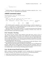
JUNOS displays the Hello timers in millisecond resolution using the show isis
interface detail operational level command.
JUNOS command output
hannes@Frankfurt> show isis interface detail
IS-IS interface database:
so-0/1/2.0
Index: 67, State: 0x6, Circuit id: 0x1, Circuit type: 3
LSP interval: 100 ms, CSNP interval: 5 s
Level Adjacencies Priority Metric Hello (s) Hold (s) Designated
Router
1 1 64 10 0.333 1
2 1 64 10 0.333 1
The JUNOS interface multiplier is hard coded (meaning it cannot be changed) to a
value of 3. A hold-timer of 1 second therefore results in a Hello interval of 333 ms, which
is the lowest Hello interval possible on JUNOS.
Relying on Hellos puts an upper boundary of 1 second to the detection time following
a link-failure on the routing protocols. But by tracking an interface state, routers can
detect the liveliness state much more quickly.
5.6.2 Interface Tracking
The chipsets that drive modern router interfaces report link errors, such as a loss of
signal, to the routing sub-system within a few milliseconds. For high-speed detection,
therefore, optical interfaces are the best choice. However, there are still similar prob-
lems, as illustrated in Figure 5.10. If there are active elements in the middle of the trans-
mission chain, then local errors are not propagated downstream and the receiving router
does not detect that the light went out.
SONET/SDH offers a true advantage over other physical media like Ethernet, which
do not propagate local errors to downstream Network Elements.

Many Protocols like Frame Relay and ATM also include their own Local Management
Interface (LMI) protocol which performs link-layer keep-alive checking, and so on.
Unfortunately there is still no LMI-like protocol for Ethernet. Bi-directional fault detec-
tion attempts make a neutral liveliness-checking protocol available.
5.6.3 Bi-directional Fault Detection (BFD)
BFD is defined in draft-katz-ward-bfd-01, and its encoding rules are documented in
draft-katz-ward-bfd-v4v6-1hop-00. BFD is an answer to the following problems:
•
Link-Layer neutral high frequency keep-alive protocol
•
Offload high frequency keep-alive processing from the IGP Layer
Neighbour Liveliness Detection 137
138 5. Neighbour Discovery and Handshaking
•
Support sub-second timers on behalf of protocols that cannot
•
Negotiate timers dynamically
The BFD protocol, unlike many other protocols, includes no auto-neighbour discov-
ery. It has client software instead, typical of the IP routing protocols, and based on the
detected IGP neighbours. The IGP asks the BFD module to set up a BFD session to the
Link IP addresses of the provided neighbours.
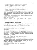
BFD is (at time of writing this book) only available for JUNOS. The first release with
support for BFD is JUNOS 6.1 onwards. The configuration of BFD is a property of the
interface {} stanza inside the protocols isis {} branch.
JUNOS configuration
Under the bfd-liveness-detection stanza you can configure the minimum transmit
interval plus the detection-time multiplier.
protocols {
isis {
interface so-1/2/0.0 {

bfd-liveness-detection {
minimum-interval 100;
multiplier 5;
}
}
[… ]
interface lo0.0;
}
}
In this example the router emits Hello packets at a rate of once every 100 ms. If the
neighbour does not receive BFD control packets for 500 ms, this router can declare the
origniator dead and move to an interface down state in the FSM.
BFD runs on top of IP UDP port 3784 and 3785. Port 3784 is used for control packets
and 3785 is used for Echo Mode traffic. The JUNOS implementation just supports con-
trol packets for liveliness detection. Echo Mode is envisioned for the future: the plan is
that forwarding plane software can generate that traffic and the control plane is only
needed for parameter setup.
The following Tcpdump output shows the parameters that are conveyed using the
24-bytes fixed length packet.
Tcpdump output
The BFD protocol runs on top of UDP port 3784 and 3785. It is meant as a high frequency
keep-alive mechanism which augments routing protocols that do not have sub-second
timer support.
09:32:30.884968 IP 172.16.223.236.3784 > 172.16.223.235.3784: BFDv0,
length: 24
Control, Flags: [I Hear You], Diagnostic: Control Detection
Time Expired (0x01)
Detection Timer Multiplier: 5 (500 ms Detection time),
BFD Length: 24
My Discriminator: 0x00000001, Your Discriminator: 0x00000002

Desired min Tx Interval: 100 ms
Required min Rx Interval: 200 ms
Required min Echo Interval: 0 ms
Session state transactions are provided using the Flag contents. The Desired/
Required Timer Fields are used for negotiating a common timer that both peers can
accept. The pair of discriminators is necessary to multiplex several sessions between a
pair of hosts.
After BFD has been enabled on both sides, one can verify if a BFD-capable neighbour
has been found on the other end and if the BFD session is Up. The show bfd ses-
sion command displays the session state.
JUNOS command output
Using the show bfd session command you can display the current state and details of
the active BFD sessions.
hannes@Frankfurt> show bfd session extensive
Transmit
Address State Interface Detect Time Interval Multiplier
172.16.223.236 Up so-0/1/2.0 1.000 0.100 5
Client ISIS L1, TX interval 0.100, RX interval 0.100, multiplier 5
Client ISIS L2, TX interval 0.100, RX interval 0.100, multiplier 5
Session up time 12:34:22, previous down time 00:00:06
Local diagnostic CtlExpire, remote diagnostic None
Remote heard, hears us
Min async interval 0.100, min slow interval 1.000
Adaptive async tx interval 0.100, rx interval 0.200
Local min tx interval 0.100, min rx interval 0.100, multiplier 5
Remote min tx interval 0.100, min rx interval 0.100, multiplier 5
Local discriminator 1, remote discriminator 2
Echo mode disabled/inactive
1 sessions, 2 clients
Cumulative transmit rate 10.0 pps, cumulative receive rate 5.0 pps

BFD is likely to become the dominant keep-alive protocol due its open implemen-
tation. It is expected to even be the protocol of choice between routers and servers.
For server applications like voice-over IP or financial applications there are open-source
BFD implementations for hosts available.
Neighbour Liveliness Detection 139
5.7 Summary
IS-IS adjacency processing has changed over the years. It started out with simple 2-way
finite state machines and, due to the underlying problems of not detecting half-broken
links, it quickly evolved to a 3-way FSM. It is remarkable that the defects of the under-
lying protocol have been solved with just the addition of an optional Adjacency State
TLV. Reliably detecting that a neighbour is Up or Down is not enough for today’s ser-
vice provider environments. On the one hand the implementation has to be slow enough
to protect the network from flapping adjacencies that are propagated through the network –
on the other hand there is a need for quick keep-alive detection mechanisms. Due to the
rise of Ethernet as popular core-facing interface technology, an LMI-like protocol like
Bi-directional Fault Detection (BFD) had to be designed. The application of BFD to
serve as an IGP detection protocol is just the start. It is expected that BFD will be used
for other network protocols or other environments like application keep-alive detection
for mission-critical servers.
140 5. Neighbour Discovery and Handshaking
6
Generating, Flooding and Ageing LSPs
141
Unlike distance vector protocols, such as RIP, link-state routing protocols, such as OSPF
and IS-IS, don’t tell only their neighbours about the topology of the network. Link-state
protocols distribute both their IP reachability and topological view far beyond their adja-
cent neighbours, ultimately flooding this information to all routers in an area.
To keep the reachability information in the network current, link-state protocols need
to have a basic set of functions available that can be used to originate, distribute and
finally revoke, or time-out topology information. In IS-IS-speak, that piece of topology

information is encoded in a link-state protocol data unit (LSP). This chapter covers these
functions and the surrounding network events th at cause the IS-IS protocol to generate,
flood and finally age LSPs.
Link-state routing protocols such as IS-IS follow a paradigm that can best be described
as distributed databases with local computation, which is quite different to the way other
common routing protocols like RIP and BGP work. Distributed databases are discussed
in more detail in the following section.
6.1 Distributed Databases
Before explaining how a distributed database works, first consider what a localized data-
base looks like and how routing protocols use it. Localized databases mean that every
router has its own local view of the network and does not know the exact topology of the
network as a whole. This is like a tourist in a foreign city having no clue about what the
overall topology of the city (the street layout) looks like. All the tourist has is a local view
of the places and streets that are next to the tourist’s immediate location. This makes it
very difficult to find the best path to a landmark or museum, and in the worst case situation,
the tourist has to try out several paths, being careful not to circle around the same locations.
Localized databases work the same way. In contrast, a distributed database approach
works differently: here all of the routers share common information about what the network
looks like. If the tourist in the example has got lost, a distributed database map would give
them a more complete map of the best way to get to a particular destination in the city (or
in this case, the network).
How does IS-IS compute the map of the network? If each router just contributes its
local view to its neighbours, and if that information can be shared among all the routers
in a network, then each will ultimately have a global map of the network. Link-state rout-
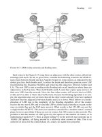
ing protocols, such as IS-IS, work like a jigsaw puzzle, as shown in Figure 6.1. Each
router in the figure represents one piece of the puzzle, and if all of the puzzle pieces are
present, then each router can start to put the puzzle together to acquire an understanding
of what the big picture looks like. The collection of puzzle pieces is called the link-state
database. IS-IS has a number of techniques called flooding and synchronizing to get a
complete map of the network. In this chapter, you will learn about the individual puzzle

pieces, which are called link-state protocol data units (LSPs), and how IS-IS distributes
the information they contain.
IS-IS, by default, tries to acquire two maps from its neighbours and therefore maintains
two databases to store topology-related information. Information for the first map, which
typically represents the topology inside the close collection of routers, called a point-
of-presence (POP), is stored in the Level 1 (L1) database. Sticking with the lost tourist
example, think of this as just a local map that guides you around the next few streets. The
second map, which typically represents the backbone structure of the network, is stored
142 6. Generating, Flooding and Ageing LSPs
Pennsauken
Frankfurt
London
Washington
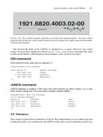
NewYork
Paris
FIGURE 6.1. A distributed link-state database is like a jigsaw puzzle
Distributed Databases 143
in the Level 2 (L2) database. This would best compare to a nationwide map where all the
freeways and highways are shown. You can take a quick look into both of these link-state
databases to find out exactly which puzzle pieces the database holds by issuing a show
isis database command on both the IOS and JUNOS software platforms.
IOS command output
The contents of the IS-IS link-state database can be displayed using the show isis
database command:
Amsterdam# show isis database
[… ]
IS-IS Level-1 Link State Database:
LSPID LSP Seq Num LSP Checksum LSP Holdtime ATT/P/OL
New-York.00-00 0x00002fac 0xC24F 60128 1/0/0
[… ]

IS-IS Level-2 Link State Database:
LSPID LSP Seq Num LSP Checksum LSP Holdtime ATT/P/OL
LINX-gw.00-00 0x00000128 0xB8EF 36163 0/0/1
LINX-gw.01-00 0x00000128 0x455A 42001 0/0/0
VIX-gw.00-00 0x00000123 0xEFC1 5023 0/0/0
[… ]
The output shows you one “puzzle piece” of information in each line. Each LSP is
uniquely identified by its LSP-ID. The exact format of the LSP-ID will be discussed later
in this chapter. All that is important for now is that it says something about the router that
originated that LSP. The sequence number is a kind of version field that tells receivers
which information is more recent. The checksum enables to check at the receiver if the
LSP has been corrupted during its long way through the network. Finally, hold-time and
the ATT/P/OL gives some information about the validity of that information and how
long it will be valid, and just like a passport it has an expiration date.
JUNOS command output
In the JUNOS software, you can display the IS-IS database using the show isis data-
base command. Watch for an inconsistency between the LSPs being sent and received,
as this is a problem indication:
hannes@New-York> show isis database
IS-IS level 1 link-state database:
LSP ID Sequence Checksum Lifetime Attributes
New-York.00-00 0x2fac 0xc24f 62063 L1 Attached
[… ]
4 LSPs
IS-IS level 2 link-state database:
LSP ID Sequence Checksum Lifetime Attributes
LINX-gw.00-00 0x128 0xb8ef 36063 L1 L2 Overload
LINX-gw.01-00 0x128 0x455a 41901 L1 L2
VIX-gw.00-00 0x123 0xefc1 4922 L1 L2
[… ]

12 LSPs
The JUNOS software output contains similar information to the IOS software output.
The only difference is the little bit more detailed breakdown of the so-called attribute
typeblock, which will be discussed later in this chapter. As far as the attribute typeblock
is concerned, the JUNOS output is more verbose than the IOS equivalent.
Based on the information in the two link-state databases for L1 and L2, each router in
an IS-IS network computes the topology of the network independently of every other
router. This principle of independent router operation is called local computation. This is
the topic of the next discussion.
6.2 Local Computation
Routing protocols, such as RIP or BGP, compute the best path through a network in a dis-
tributed fashion. That is, no single RIP or BGP router knows what the other routers know
about the route, and this is a real limitation. For instance, each time a RIP router passes on
a route to its neighbour, the route gets a worse value. This “worseness” is indicted in a
metric field, which represents the hop-count (number of routers) that a router is away from
the router attached to the source sub-net. In Figure 6.2 the sub-net 192.168.1/24 is directly
connected to RIP Router #1. Router #1 reports the sub-net to its neighbours with a hop
count of 1. Router #2 learns the sub-net with a metric of 1 and reports it further to the right
side of the figure after incrementing the metric field by one. The routing update therefore
arrives at Router #3 with a metric of 2. But Router #1 has no idea what value this route has
on Router #3. RIP routing illustrates how a distributed computation scheme works.
IS-IS utilizes a totally different way of calculating routing information. Before the route
calculation takes place, all IS-IS routers distribute the information about the local views
of the routers to each other. Intermediate routers along the way must not change these
views (represented in the LSPs). After this distribution (flooding), a common route-
calculation scheme, which in IS-IS is called the shortest path first (SPF) algorithm, is
applied. Note that each router computes the routes independently from every other router.
144 6. Generating, Flooding and Ageing LSPs
192.168.1/24
…

RIP Router 1 RIP Router 2 RIP Router 3 RIP Router 4
192.168.1/24 (1) 192.168.1/24 (2) 192.168.1/24 (3)
…
192.168.1/24 (4)
…
…
FIGURE 6.2. RIP calculates the metric in a distributed fashion
Local Computation 145
You can watch the result of the SPF calculation by issuing a show ip route isis com-
mand on IOS platforms and a show isis route command on Juniper Network routers.
In IOS, you cannot see the entire results of the SPF calculation – all you can see are
the results that make it into the main routing table. That excludes redundant routers that
happen to be in both IS-IS levels. The IS-IS learned routes that are active in the routing
table can be displayed using the show ip route isis command.
IOS command output
Amsterdam#show ip route isis
[… ]
i L1 192.168.0.55 [115/10] via 172.16.144.2, POS3/0
i L1 192.168.0.57 [115/10] via 172.16.144.2, POS4/0
i L2 192.168.1.122 [115/10] via 172.16.177.18, GigabitEthernet3/0
[… ]
The output tells us basically what routes (second column) did get installed in the local
routing and forwarding tables. Each line contains information about a single route. The
first column shows the level. The numbers in the brackets after the route give informa-
tion about the weight or, as it is called in Cisco IOS speak, the administrative distance of
the routing protocol that inserted this route into the routing table (in this case, IS-IS).
After the “via” statement the IP address of a locally connected router appears (the next-
hop). Finally the end of each line gives the physical interface through which the next-hop
can be reached and this is how packets to this destination will leave the router.
In the JUNOS software, you can display both the immediate results from the SPF calcu-

lation as well as the routes installed in the routing table. The SPF results are displayed using
the show isis route command. The IS-IS learned routes that are active in the main
routing table can be displayed using the show route protocol isis command.
JUNOS software command output
hannes@Pennsauken> show isis route
IS-IS routing table Current version: L1: 0 L2: 485
Prefix L Version Metric Type Interface Via
172.16.44.248/30 2 485 61770 int so-3/0/0.0 London
192.168.49.5/32 2 485 67850 int so-3/0/0.0 London
192.168.49.67/32 2 485 67860 int so-3/0/0.0 London
192.168.52.177/32 2 485 127850 int so-3/0/0.0 Frankfurt
192.168.54.164/32 2 485 128510 int so-3/0/0.0 Frankfurt
172.16.176.0/24 2 485 121770 int so-3/0/0.0 Frankfurt
172.16.176.32/30 2 485 127830 int so-3/0/0.0 New-York
172.16.176.60/30 2 485 123790 int so-3/0/0.0 New-York
[… ]
The format of the output is one route entry per line. The first column contains the route
and the second column contains information about the level where this route did result
from. The version field is just an internal number that tells you how the SPF run number
based upon this route was calculated. The version field is typically not interesting in
troubleshooting networks. The metric tells the distance relative to the local router of the
prefix. Next is an indication whether the route is internal or external. Typically all the
routes are internal unless routes have been injected from other routing protocols into the IS-
IS database. Finally, the interface where the traffic leaves the router is displayed, plus the
forwarding router’s name.
JUNOS software command output
hannes@Pennsauken> show route protocol isis
inet.0: 118243 destinations, 246129 routes (118243 active,
0 holddown, 0 hidden)
+ = Active Route, - = Last Active, * = Both

172.16.44.248/30 *[IS-IS/18] 4d 12:57:11, metric 41550, tag 2
> to 172.16.5.93 via so-3/2/0.0
192.168.49.5/32 *[IS-IS/18] 2d 07:26:54, metric 67850, tag 2
> to 172.16.5.93 via so-2/3/0.0
192.168.49.67/32 *[IS-IS/18] 1d 20:01:28, metric 67860, tag 2
> to 172.16.5.93 via so-7/0/0.0
[… ]
In the show route protocol isis output we can see a subset of routes that got
displayed in show isis routes. Those are the routes that competed for installation in
the routing table with other routing protocols that may have had similar information;
however, the routes in this table are the ones that have won. In JUNOS the level of routes
is displayed in the tag field – a tag 2 means that this is a Level 2 route. The number in the
brackets is a similar value to the administrative distance for IOS platforms, called sim-
ply the route preference. The to and via keywords indicate the next-hop and the outgoing
interface.
The universal transport vehicle to build the IS-IS database map is called a link-state
protocol data unit or LSP for short, which is another OSI-speak word for link-state
packet. In the following sections, you will see what information an LSP contains, how
the LSP gets distributed, and how LSPs get throttled when the network is busy.
6.3 LSPs and Revision Control
The information element that transports IS-IS-related information to populate all the
routers’ link-state databases is called the link-state PDU or LSP. Each router in an IS-IS
network generates at least one LSP that describes, as the name implies, the current state
of the links to other routers. Actually, an LSP conveys more than just the state of the links
or circuits on the router. Routers use LSPs as a kind of envelope to get different types of
information elements such as IP routes, checksums and even router names across to other
routers. LSPs need to be accurate and up-to-date. If, for example, a link between a pair
of routers goes down, both routers must immediately tell the other routers in the network
146 6. Generating, Flooding and Ageing LSPs