Scalable voip mobility intedration and deployment- P5 potx

38 Chapter 2
www.newnespress.com
PSTN integration as the standard case (Skype’s landline telephone services can be thought
of more as special cases) has allowed it to be optimized for better voice quality in a lossy
environment.
Skype is unlikely to be useful in current voice mobility deployments, so it will not be
mentioned much further in this book. However, Skype will always be found performing
somewhere within the enterprise, and so its usage should be understood. As time progresses,
it may be possible that people will have worked out a more full understanding of how to
deploy Skype in the enterprise.
2.2.5 Polycom SpectraLink Voice Priority (SVP)
Early in the days of voice over Wi-Fi, a company called SpectraLink—now owned by
Polycom—created a Wi-Fi handset, gateway, and a protocol between them to allow the
phones to have good voice quality, when Wi-Fi itself did not yet have Wi-Fi Multimedia
(WMM) quality of service. SVP runs as a self-contained protocol, for both signaling and
bearer traffic, over IP, using a proprietary IP type (neither UDP nor TCP) for all of the traffic.
SVP is not intended to be an end-to-end signaling protocol. Rather, like Cisco’s SCCP, it is
intended to bridge between a network server that speaks the real telephone protocol and the
proprietary telephone. Therefore, SCCP and SVP have a roughly similar architecture. The
major difference is that SVP was designed with wireless in mind to tackle the early quality-
of-service issues over Wi-Fi, whereas SCCP was designed mostly as a way of simplifying
the operation of phone terminals over wireline IP networks.
Figure 2.6 shows the SVP architecture. The SVP system integrates into a standard IP PBX
deployment. The SVP gateway acts as the location for the extensions, as far as the PBX is
concerned. The gateway also acts as the coordinator for all of the wireless phones. SVP
phones connect with the gateway, where they are provisioned. The job of the SVP gateway
is to perform all of the wireless voice resource management of the network. The SVP
performs the admission control for the phones, being configured with the maximum number
of phones per access point and denying phones the ability to connect to it through access
points that are oversubscribed. The SVP server also engages in performing timeslice
coordination for each phone on a given access point.

This timeslicing function makes sense in the context of how SVP phones operate. SVP
phones have proprietary Wi-Fi radios, and the protocol between the SVP gateway and the
phone knows about Wi-Fi. Every phone reports back what access point it is associated to.
When the phone is placed into a call, the SVP gateway and the phone connect their bearer
channels. The timing of the packets sent by the phone is such that it is directly related to
the timing of the phone sent by the gateway. Both the phone and the gateway have specific
requirements on how the packets end up over the air. This, then, requires that the access
points also be modified to be compatible with SVP. The role of the access point is to
Voice Mobility Technologies 39
www.newnespress.com
PBX
SVP Phone
Media Gateway
SVP Gateway
Access Point
Public Switched Telephony Network (PSTN)
Any Supported Voice
Signaling and Bearer Traffic
SVP Proprietary
Signaling and Bearer Traffic
Telephone Lines
Gateway
Gateway
ExtensionsDial Plan
Figure 2.6: SVP Architecture
40 Chapter 2
www.newnespress.com
dutifully follow a few rules which are a part of the SVP protocol, to ensure that the packets
access the air at high priority and are not reordered. There are additional requirements for
how the access point must behave when a voice packet is lost and must be retransmitted by

the access point. By following the rules, the access point allows the client to predict how
traffic will perform, and thus ensures the quality of the voice.
SVP is a unique protocol and system, in that it is designed specifically for Wi-Fi, and in
such a way that it tries to drive the quality of service of the entire SVP system on that
network through intelligence placed in a separate, nonwireless gateway. SVP, and
Polycom SpectraLink phones, are Wi-Fi-only devices that are common in hospitals and
manufacturing, where there is a heavy mobile call load inside the building but essentially no
roaming required to outside.
2.2.6 ISDN and Q.931
The ISDN protocol is where telephone calls to the outside world get started. ISDN is the
digital telephone line standard, and is what the phone company provides to organizations
that ask for digital lines. By itself, ISDN is not exactly a voice mobility protocol, but
because a great number of voice calls from voice mobility devices must go over the public
telephone network at some point, ISDN is important to understand.
With ISDN, however, we leave the world of packet-based voice, and look at tightly timed
serial lines, divided into digital circuits. These circuits extend from the local public
exchange—where analog phone lines sprout from before they run to the houses—over the
same types of copper wires as for analog phones. The typical ISDN line that an enterprise
uses starts from the designation T1, referring to a digital line with 24 voice circuits
multiplexed onto it, for 1536kbps. The concept of the T1 (also known, somewhat more
correctly, as a DS1, with each of the 24 digital circuits known as DS0s) is rather simple.
The T1 line acts as a constant source or sink for these 1536kbps, divided up into the 24
channels of 64kbps each. With a few extra bits for overhead, to make sure both sides agree
on which channel is which, the T1 simply goes in round-robin order, dedicating an eight-bit
chunk (the actual byte) for the first circuit (channel), then the second, and so on. The vast
majority of traffic is bearer traffic, encoded as standard 64kbps audio, as you will learn
about in Section 2.3. The 23 channels dedicated for bearer traffic are called B channels.
As for signaling, an ISDN line that is running a signaling protocol uses the 24th line, called
the D channel. This runs as a 64kbps network link, and standards define how this
continuous serial line is broken up into messages. The signaling that goes over this channel

usually falls into the ITU Q.931 protocol.
Q.931’s job is to coordinate the setting up and tearing down of the independent bearer
channels. To do this, Q.931 uses a particular structure for their messages. Because Q.931
Voice Mobility Technologies 41
www.newnespress.com
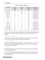
Table 2.18 shows the basic format of the Q.931 message. The protocol discriminator is
always the number 8. The call reference refers to the call that is being referred to, and is
determined by the endpoints. The information elements contain the message body, stored in
an extensible yet compact format.
The message type is encompasses the activities of the protocol itself. To get a better sense
for Q.931, the message types and meanings are:
• SETUP: this message starts the call. Included in the setup message is the dialed number,
the number of the caller, and the type of bearer to use.
• CALL PROCEEDING: this message is returned by the other side, to inform the caller
that the call is underway, and specifies which specific bearer channel can be used.
• ALERTING: informs the caller that the other party is ringing.
• CONNECT: the call has been answered, and the bearer channel is in use.
• DISCONNECT: the phone call is hanging up.
• RELEASE: releases the phone call and frees up the bearer.
• RELEASE COMPLETE: acknowledges the release.
There are a few more messages, but it is pretty clear to see that Q.931 might be the simplest
protocol we have seen yet! There is a good reason for this: the public telephone system
is remarkably uniform and homogenous. There is no reason for there to be flexible or
complicated protocols, when the only action underway is to inform one side or the other of
a call coming in, or choosing which companion bearer lines need to be used. Because Q.931
is designed from the point of view of the subscriber, network management issues do not
need to be addressed by the protocol. In any event, a T1 line is limited to only 64kbps for
the entire call signaling protocol, and that needs to be shared across the other 23 lines.
Digital PBXs use IDSN lines with Q.931 to communicate with each other and with the
public telephone networks. IP PBXs, with IP links, will use one of the packet-based

signaling protocols mentioned earlier.
Table 2.18: Q.931 Basic Format
Protocol
Discriminator
Length of Call
Reference
Call Reference Message Type Information
Elements
1 byte 1 byte 1–15 bytes 1 byte
variable
can run over any number of different protocols besides ISDN, with H.323 being the other
major one, the descriptions provided here will steer clear of describing how the Q.931
messages are packaged.
42 Chapter 2
www.newnespress.com
2.2.7 SS7
Signaling System #7 (SS7) is the protocol that makes the public telephone networks operate,
within themselves and across boundaries. Unlike Q.931, which is designed for simplicity,
SS7 is a complete, Internet-like architecture and set of protocols, designed to allow call
signaling and control to flow across a small, shared set of circuits dedicated for signaling,
freeing up the rest of the circuits for real phone calls.
SS7 is an old protocol, from around 1980, and is, in fact, the seventh version of the
protocol. The entire goal of the architecture was to free up lines for phone calls by
removing the signaling from the bearer channel. This is the origin of the split signaling and
bearer distinction. Before digital signaling, phone lines between networks were similar to
phone lines into the home. One side would pick up the line, present a series of digits as
tones, and then wait for the other side to route the call and present tones for success, or
a busy network. The problem with this method of in-band signaling was that it required
having the line held just for signaling, even for calls that could never go through. To free up
the waste from the in-band signaling, the networks divided up the circuits into a large pool

of voice-only bearer lines, and a smaller number of signaling-only lines. SS7 runs over the
signaling lines.
It would be inappropriate here to go into any significant detail into SS7, as it is not seen as
a part of voice mobility networks. However, it is useful to understand a bit of the
architecture behind it.
SS7 is a packet-based network, structured rather like the Internet (or vice versa). The phone
call first enters the network at the telephone exchange, starting at the Service Switching
Point (SSP). This switching point takes the dialed digits and looks for where, in the
network, the path to the other phone ought to be. It does this by sending requests, over the
signaling network, to the Service Control Point (SCP). The SCP has the mapping of user-
understandable telephone numbers to addresses on the SS7 network, known as point codes.
The SCP responds to the SSP with the path the call ought to take. At this point, the switch
(SSP) seeks out the destination switch (SSP), and establishes the call. All the while, routers
called Signal Transfer Points (STPs) connect physical links of the network and route the
SS7 messages between SSPs and SCPs.
The interesting part of this is that the SCP has this mapping of phone numbers to real,
physical addresses. This means that phone numbers are abstract entities, like email
addresses or domain names, and not like IP addresses or other numbers that are pinned
down to some location. Of course, we already know the benefit of this, as anyone who has
ever changed cellular carriers and kept their phone number has used this ability for that
mapping to be changed. The mapping can also be regional, as toll-free 800 numbers take
advantage of that mapping as well.
Voice Mobility Technologies 43
www.newnespress.com
Voice, as you know, starts off as sound waves (Figure 2.7). These sound waves are picked
up by the microphone in the handset, and are then converted into electrical signals, with the
voltage of the signal varying with the pressure the sound waves apply to the microphone.
The signal (see Figure 2.8) is then sampled down into digital, using an analog-to-digital
converter
. Voice tends to have a frequency around 3000 Hz. Some sounds are higher—

music especially needs the higher frequencies—but voice can be represented without
significant distortion at the 3000Hz range. Digital sampling works by measuring the voltage
of the signal at precise, instantaneous time intervals. Because sound waves are, well, wavy,
as are the electrical signals produced by them, the digital sampling must occur at a high
enough rate to capture the highest frequency of the voice. As you can see in the figure, the
signal has a major oscillation, at what would roughly be said is the pitch of the voice. Finer
variations, however, exist, as can be seen on closer inspection, and these variations make up
the depth or richness of the voice. Voice for telephone communications is usually limited
to 4000 Hz, which is high enough to capture the major pitch and enough of the texture to
make the voice sound human, if a bit tinny. Capturing at even higher rates, as is done on
compact discs and music recordings, provides an even stronger sense of the original voice.
Sampling audio so that frequencies up to 4000 Hz can be preserved requires sampling the
signal at twice that speed, or 8000 times a second. This is according to the Nyquist
Sampling Theorem. The intuition behind this is fairly obvious. Sampling at regular intervals
is choosing which value at those given instants. The worst case for sampling would be if
Phone
Talking
Person
Analog-to-Digital
Converter
Voice Encoder Packetizer Radio
Figure 2.7: Typical Voice Recording Mechanisms
2.3 Bearer Protocols in Detail
The bearer protocols are where the real work in voice gets done. The bearer channel carries
the voice, sampled by microphones as digital data, compressed in some manner, and then
placed into packets which need to be coordinated as they fly over the networks.
44 Chapter 2
www.newnespress.com
Time
Intensity

Intensity
Intensity
0
0
0
Figure 2.8: Example Voice Signal, Zoomed in Three Times
one sampled a 4000 Hz, say, sine wave at 4000 times a second. That would guarantee to
provide a flat sample, as the top pair of graphs in Figure 2.9 shows. This is a severe case of
undersampling, leading to aliasing effects. On the other hand, a more likely signal, with a
more likely sampling rate, is shown in the bottom pair of graphs in the same figure. Here,
the overall form of the signal, including its fundamental frequency, is preserved, but most
of the higher-frequency texture is lost. The sampled signal would have the right pitch, but
would sound off.
The other aspect to the digital sampling, besides the 8000 samples-per-second rate, is the
amount of detail captured vertically, into the intensity. The question becomes how many bits
Voice Mobility Technologies 45
www.newnespress.com
Time
Intensity
Intensity
Original Signal
Original Signal
SampledSignal
0
0
Intensity
Sampled Signal
0
Intensity
0

Figure 2.9: Sampling and Aliasing
46 Chapter 2
www.newnespress.com
of information should be used to represent the intensity of each sample. In the quantization
process, the infinitely variable, continuous scale of intensities is reduced to a discrete,
quantized scale of digital values. Up to a constant factor, corresponding to the maximum
intensity that can be represented, the common value for quantization for voice is to 16 bits,
for a number between –2
15
= –32,768 to 2
15
– 1 = 32,767.
The overall result is a digital stream of 16-bit values, and the process is called pulse code
modulation (PCM), a term originating in other methods of encoding audio that are no
longer used.
2.3.1 Codecs
The 8000 samples-per-second PCM signal, at 16 bits per sample, results in 128,000 bits per
second of information. That’s fairly high, especially in the world of wireline telephone
networks, in which every bit represented some collection of additional copper lines that
needed to have been laid in the ground. Therefore, the concept of audio compression was
brought to bear on the subject.
An audio or video compression mechanism is often referred to as a codec, short for coder-
decoder. The reason is that the compressed signal is often thought of as being in a code,
some sequence of bits that is meaningful to the decoder but not much else. (Unfortunately,
in anything digital, the term code is used far too often.)
The simplest coder that can be thought of is a null codec. A null codec doesn’t touch
the audio: you get out what you put in. More meaningful codecs reduce the amount of
information in the signal. All lossy compression algorithms, as most of the audio and video
codecs are, stem from the realization that the human mind and senses cannot detect every
slight variation in the media being presented. There is a lot of noise that can be added, in

just the right ways, and no one will notice. The reason is that we are more sensitive to
certain types of variations than others. For audio, we can think of it this way. As you drive
along the highway, listening to AM radio, there is always some amount of noise creeping
in, whether it be from your car passing behind a concrete building, or under power lines, or
behind hills. This noise is always there, but you don’t always hear it. Sometimes, the noise
is excessive, and the station becomes annoying to listen to or incomprehensible, drowned
out by static. Other times, however, the noise is there but does not interfere with your
ability to hear what is being said. The human mind is able to compensate for quite a lot
of background noise, silently deleting it from perception, as anyone who has noticed the
refrigerator’s compressor stop or realized that a crowded, noisy room has just gone quiet
can attest to. Lossy compression, then, is the art of knowing which types of noise the
listener can tolerate, which they cannot stand, and which they might not even be able
to hear.
Voice Mobility Technologies 47
www.newnespress.com
(Why noise? Lossy compression is a method of deleting information, which may or may
not be needed. Clearly, every bit is needed to restore the signal to its original sampled state.
Deleting a few bits requires that the decompressor or the decoder restore those deleted bits’
worth of information on the other end, filling them in with whatever the algorithm states is
appropriate. That results in a difference of the signal, compared to the original, and that
difference is distortion. Subtract the two signals, and the resulting difference signal is the
noise that was added to the original signal by the compression algorithm. One only need
amplify this noise signal to appreciate how it sounds.)
2.3.1.1 G.711 and Logarithmic Compression
The first, and simplest, lossy compression codec for audio that we need to look at is called
logarithmic compression. Sixteen bits is a lot to encode the intensity of an audio sample.
The reason why 16 bits was chosen was that it has fine enough detail to adequately
represent the variations of the softer sounds that might be recorded. But louder sounds do
not need such fine detail while they are loud. The higher the intensity of the sample, the
more detailed the 16-bit sampling is relative to the intensity. In other words, the 16-bit

resolution was chosen conservatively, and is excessively precise for higher intensities. As
it turns out, higher intensities can tolerate even more error than lower ones—in a relative
sense, as well. A higher-intensity sample may tolerate four times as much error as a signal
half as intense, rather than the two times you would expect for a linear process. The reason
for this has to do with how the ear perceives sound, and is why sound levels are measured
in decibels. This is precisely what logarithmic compression does. Convert the intensities to
decibels, where a 1 dB change sounds roughly the same at all intensities, and a good half of
the 16 bits can be thrown away. Thus, we get a 2 : 1 compression ratio.
The ITU G.711 standard is the first common codec we will see, and uses this logarithmic
compression. There are two flavors of G.711: µ-law and A-law. µ-law is used in the United
States, and bases its compression on a discrete form of taking the logarithm of the incoming
signal. First, the signal is reduced to a 14-bit signal, discarding the two least-significant bits.
Then, the signal is divided up into ranges, each range having 16 intervals, for four bits, with
twice the spacing as that of the next smaller range. Table 2.19 shows the conversion table.
The number of the interval is where the input falls within the range. 90, for example, would
map to 0xee, as 90 − 31 = 59, which is 14.75, or 0xe (rounded down) away from zero, in
steps of four. (Of course, the original 16-bit signal was four times, or two bits, larger, so
360 would have been one such 16-bit input, as would have any number between 348 and
363. This range represents the loss of information, as 363 and 348 come out the same.)
A-law is similar, but uses a slightly different set of spacings, based on an algorithm that is
easier to see when the numbers are written out in binary form. The process is simply to take
the binary number and encode it by saving only four bits of significant digits (except the