Scalable voip mobility intedration and deployment- P14 pptx

130 Chapter 5
www.newnespress.com
The formula for the channels to frequencies is 2.407GHz + 0.5GHz * channel for the
2.4GHz band, and the simpler to remember 5GHz + 0.5GHz * channel for the 5GHz band.
The only channels that are in the 2.4GHz band are channels 1–14. Everything else is in the
5GHz band. Therefore, channel 36 is 5.18GHz, and channel 100 is 5.50GHz.
The total number of channels is large, but many factors reduce the number that can be
practically used. First to note is that the 2.4GHz band, where 802.11b and 802.11g run, only
has three nonoverlapping channels (four in Japan) to choose from. Unfortunately, the eleven
channel numbers available in the United States gives the false impression of 11 independent
channels, and to this day there exist some Wi-Fi deployments that mistakenly use all 11
channels, causing an RF nightmare. To avoid overlapping channels, adjacent channel
selections need to be four channel numbers apart. Therefore, channels 1 and 5 do not
overlap. In the 2.4GHz band, custom usually spreads the channels out even a bit further,
and using only channels 1, 6, and 11 is recommended. The authors of the standard
recognized the problem the overlap causes, and, for the 5GHz band, disallowed overlap by
preventing devices from using the intermediate channels. Therefore, no channels in the
5GHz band overlap, when it comes to 20MHz channels. (40MHz channels are an exception,
and will be discussed in the section on 802.11n, Section 5.5.3.)
The unlicensed spectrum was originally designed for, and still is allocated to, other uses
besides Wi-Fi. The 2.4GHz band was created to allow, in part, for microwave ovens to emit
radio noise as they operate, as it is impractical to completely block their radio emissions.
Because that noise prevented being able to provide the protections from interference that
licensed bands have, the regulatory agencies allowed inventors to experiment providing
other services in this band. And so began 802.11. The 5GHz band is, in theory, more set
aside from radiation. Except for the top 5.8GHz ISM band, the 5GHz range was
designed for communications devices. However, interference still exists. One primary
source, and the one important from a regulatory point of view, is radar. Radars operate in
the same 5GHz band. Because the radars are given priority, Wi-Fi devices in much of the
5GHz band are required to either be used indoors only, or to detect when a radar is present
and shut down or change channels. This last ability is known as dynamic frequency

selection (DFS). This is not a feature or benefit, per se, but a requirement from the various
governments. DFS complicates the handoff process significantly, and will be further
explored in Section 6.2.2.
5.3.2 Radio Basics
Radio technology can seem rather complicated. Wi-Fi transmitters emit power at a given
strength, but receivers have to be able to correctly decode those signals at power levels up to a
billion times weaker, just for normal wireless networks to work. This incredible swing in
power levels requires quite a bit of smarts in both the definitions of the signals and in the
Introduction to Wi-Fi 131
www.newnespress.com
designs of the radios themselves. It is impossible to describe every important concept in the
world of radios, but we will cover those concepts that have the most impact for voice mobility.
5.3.2.1 Power and Multipath
Power, or signal strength, is the amount of energy the radio pushes into the air over time.
Power is measured in watts. However, for wireless, a watt is a large value, and the receiver
usually gets signals many millions of times weaker, once the radio waves reach it.
Therefore, Wi-Fi devices tend to refer to milliwatts, or mW. To cover the wide range, the
logarithmic decibel is also used. Therefore, power can also be measured in dBm, or decibels
of milliwatts. (More formally, it can be called dBmW; however, the W for watt is usually
left off.) 0
dBm equals 1 mW. The conversion formula is P
dBm
= 10 × log
10
P
mW
, where P
dBm

is the power in dBm and P

mW
is the power in milliwatts. It is handy to remember that a 3dB
change in power is roughly equal to a two-fold change in power. Note that differences
between two dBm values are cited in dB, not in dBm. Therefore, the difference between an
18dBm and a 21dBm transmission power is referred to as 3dB. The reason is because the
difference of any logarithmic value is really a ratio of two nonlogarithmic values, and thus
21dBm −18dBm is really stating that the ratio of the two power levels is roughly 2, or that
21dBm is 2 times stronger than 18dBm. (The units of milliwatts cancel in the ratio.)
The wide difference in power levels stems from the inverse square law. In free space, space
with nothing to interfere or interact with the radio waves, the power of radio signals falls
off with the square of the distance, as the power is spread evenly across space. (The reason
why spreading power evenly causes the exponent to be 2 is that the area of a sphere grows
as the square of the distance. Picture the same amount of radiation smeared over the surface
of a sphere growing from the antenna.) This means that short amounts of distance can cause
the signal to fall off rapidly. As it turns out, when thinking about wireless, the inverse
square law should be thought of with a few modifications.
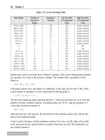
First, radio waves do not pass through all materials equally. The denser the material, the
more the radio waves are weakened. This process is called attenuation, and how much an
object attenuates is measured in the difference in power level the object causes over free
space path loss. A vacuum, and for the most part, dry air, does not attenuate radio waves,
and thus can be thought of as having 0dB of attenuation. A wooded wall might attenuate
radio waves a bit, and so might have 3dB of attenuation. A cement wall, being thicker,
might have 10dB of attenuation. The denser, thicker, or more conductive (metallic) the
material is, the higher the attenuation Figure 5.6 shows an example of signal falloff. Certain
objects are especially bad for Wi-Fi. Wire mesh, such as chicken wire lathing used in
certain plaster walls, metal paneling and ductwork, and water-containing materials tend to
cause high amounts of attenuation, as they absorb the radio waves better than dry and less
dense materials. This shows up in deployments where old buildings, plumbing, elevator
cores, and stairwells tend to disproportionately dampen the power of radio signals.
132 Chapter 5

www.newnespress.com
Second, radio signals do not travel as far at higher frequencies than at lower ones. The
higher the frequency, the more quickly signals fall off, and the more strongly they interact
with and are stopped by objects. This can be understood rather easily. AM channels on
radios tend to travel for hundreds of miles—long after you have left the city. That is
because they are very low-frequency—in the kilohertz range. AM radio waves pass through
walls, buildings, and mountains with relative ease. On the other hand, visible light only
goes through glass. That is because light is a very high-frequency radio signal—400
terahertz or higher. In Wi-Fi, this is most noticeable in the difference between 2.4GHz
(802.11bgn, referring to how 802.11n radios in the 2.4GHz band must support 802.11g and
802.11b as well) and 5GHz (802.11an), where the 5GHz radio waves may be stopped many
feet before the 2.4GHz radio waves are, depending on the environment.
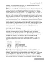
Third, radio waves reflect, and these reflections get mixed into the radio waves that are
being transmitted, amplifying or weakening the signal. This effect, known as multipath, is
caused by the constructive or destructive interference of radio waves, most often caused by
reflections from multiple surfaces (see Figure 5.7). The name “multipath” comes from how
the signal at any point in space can be thought of as the sum of radio waves bouncing as
light rays along multiple paths. Multipath is a real problem with Wi-Fi, and is difficult to
account for. That is because multipath doesn’t just increase or decrease the strength of the
signal. Radio waves travel at a fixed speed, the speed of light, and therefore those
components of a signal that are reflected from objects further away are also slightly more
delayed. The speed of light is quick—light travels at around 30 cm per nanosecond—but
nanoseconds are in the range of times that Wi-Fi signals change to carry information.
Therefore, the effect of multipath is add delayed echoes of the signal to the original signal,
increasing the distortion of the signal as well. In environments where multipath does not
Distance (feet)
Power (dBm)
0 dBm
Wall (5dB attenuation) Metal (10dB attenuation)
5 ft

10 ft
15 ft
20 ft
25 ft
30 ft
35 ft
40 ft
45 ft
50 ft
55 ft
60 ft
-10 dBm
-20 dBm
-30 dBm
-40 dBm
-50 dBm
-60 dBm
-70 dBm
-80 dBm
-90 dBm
-100 dBm
Figure 5.6: How Signals Weaken: Distance and Attenuation
Introduction to Wi-Fi 133
www.newnespress.com
Strongest Signal
Crest of wave
Trough of wave
No Signal
Figure 5.7: Two Transmitters and How the Signals Combine or Cancel
substantially distort the signals, the greater effect is that attenuation, and is actually modeled

by altering the inverse square law’s square parameter. The path loss exponent (PLE) is
usually adjusted upwards, from the value 2, to accommodate the effects of the environment
in weakening the signal over distance. Office spaces often have path loss exponents around
2.3 to 2.5. Some environments, on the other hand, such as long metallic hallways or
airplanes, have path loss exponents less than 2. No, the laws of physics are not being
violated—even the inverse square law is still absolutely correct with a PLE of 2 and only
2—but rather, the reflections from the long hallway make the environment serve as a
waveguide, and those reflections constructively interfere, or amplify the signal, more than
free space would. (The overall energy radiated out remains the same, just concentrated in
the areas with PLE less than 2 and necessarily lessened in others.)
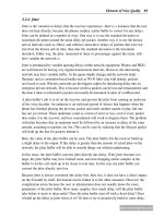
All this means that the strength of Wi-Fi signals depends heavily on the environment. The
802.11 standard has a diagram that is telling.
Figure 5.8, present in the IEEE 802.11 standard, shows the signal strengths throughout a
one-room office. The darker the color, the weaker the signal, and the lighter the color, the
stronger the signal. It is clear to see that the reflections cause intense ripple patterns across
the room. These ripples are spaced a wavelength apart, and the difference from peak to
trough is 50dB, or over one hundred thousand times the power.
134 Chapter 5
www.newnespress.com
The problem with the ripples is that they are nearly impossible to predict. This has an
impact on the performance of the wireless network.
5.3.2.2 Noise and Interference
Radio noise occurs in Wi-Fi networks from three main sources. Each source contributes to
the noise floor, which represents the background signal power level that will always be
present. Signals that can be received must be a certain power level above the noise floor, in
order for the signal to be distinct from the din. All of the major theory behind radio
reception and information transfer relate the capacity to send information, and the amount
of information that can be sent, to the ratio of the signal power level to this noise floor.
The first source of noise is the most basic and least interesting to voice mobility networks once
it is understood. Thermal noise is the noise produced in every RF frequency because of the

temperature of the world and all of the things in it. Thermal noise is a basic property of the fact
that radio waves are light, and light is radiated because of the temperature of objects. The
phenomenon that causes a piece of metal to become red when heated also causes the thermal
background radiation within the Wi-Fi bands. The noise is not only coming from the
nonradiating components in the room. The radios themselves—the antennas, the circuit paths,
and the amplifiers and active components—all themselves are injecting thermal noise in the
radio circuits. This is most important for the receiver’s circuits, as this noise is what can drown
out the weak signal coming in. In Wi-Fi networks, the noise floor tends to get no lower than
around −100dBm, measured by Wi-Fi devices. This sort of noise is expected to be random and
predictable, but predictable in how it is random. Once the thermal noise level is learned, it
should not change by more than a couple of dB as time goes on, and that variation is as much
the result of temperature variations as the Wi-Fi equipment heats up.
Figure 5.8: Signal Combination in a Room
Introduction to Wi-Fi 135
www.newnespress.com
The second source of noise comes from non-Wi-Fi devices. Microwave ovens, cordless
phones, Bluetooth devices, and industrial machinery all inject noise into the Wi-Fi bands.
Devices are allowed, by regulatory rules, to inject this noise into the ISM bands that Wi-Fi
uses, as long as the power level does not exceed certain thresholds. But intentionally
generated communications signals tend to be of greater concern, as coexistence between
different technologies in the unlicensed spectrum is mandatory, and Wi-Fi is not the only
technology. The two ISM bands, the 2.4GHz and the 5.8GHz, are where these devices
should be expected. The 5.8GHz band can especially have surprising sources of noise,
because there are outdoor applications for the 5.8GHz band, using high-power but low-
beam-width transmitters. A neighbor could easily set up such a system and interfere with a
Wi-Fi network already in place.
The third, and most important source of noise is self noise, or noise generated by Wi-Fi
from its operation. This noise always comes from neighboring access points’ devices, which
generate enough power that their signal energy reaches some of all of the devices in the
given cell. In the best case, those interfering signals may reach the devices as weak,

undecipherable power, contributing to an effective rise in the noise floor, but not necessarily
resulting in a direct change into the operation of the Wi-Fi protocol. This sort of noise is
always present in Wi-Fi networks that see more than a trivial amount of use. The more
densely deployed the network is, as a mixture of access points and the clients that use them,
the higher the noise floor will rise because of the contribution of this power. The noise floor
can rise as high as −80dBm in many networks when being used, and even higher when the
network comes under stress. In networks where the density is reasonably elevated, the effect
of the other devices is stronger than noise, as it directly affects the Wi-Fi protocol by
causing the devices to detect the distant transmissions and defer transmission. Even when
this does not happen, the bursty on-and-off nature of Wi-Fi can mean that transmissions in
progress can experience bit errors as the interference disrupts the radios themselves, without
being detected as noise or energy outright.
5.3.3 RF Planning
RF planning is designed to address the two problems of multicellular networks. The first
problem is to ensure that the coverage levels within the network are high enough that the
expected data rates, based on the minimum required signal to noise ration, can be achieved
at every useful square foot of the building or campus environment. The second problem is
to avoid the intercell interference which results from multiple devices transmitting on the air
without mitigation.
Proper RF planning is an expensive, time-consuming process. The basics of RF planning
are for the installers to predict what the signal propagation properties will be in the expected
environment. This sort of activity always requires using sophisticated RF prediction tools.
RF prediction tools operate by requiring the operator to designate the locations and RF
136 Chapter 5
www.newnespress.com
properties—attenuation, mostly—of each physical element in the building, the furniture, the
walls, the floors, and the heavy machinery. Clearly a laborious process, the operator must
copy in the location of these elements one at a time. Some tools are intelligent enough to
take CAD drawings or floor-plan maps and estimate where the walls are, but an operator is
required to verify that the guesses are not far from reality. RF planning tools then use RF

calculations, based on electromagnetic principles, to determine how much the signal is
diminished or attenuated by the environment. The planning tools need to know the transmit
power capabilities and antenna gains of all of the access points that will be deployed in the
network.
RF planning can be used this way to assist in determining where access points ought to be
located, to maximize coverage given the particular SNR requirements. Because RF planning
uses exact equations to predict the effects of the environment, it can be only as good as the
information it is given. Operators must enter the exact RF and physical properties of the
building to have a high likelihood of getting an accurate answer. For this reason, RF
planning suffers from the garbage-in-garbage-out problem. If the operator has uncertainty
about the makeup of the materials in the building, then the results of the RF plan share the
same uncertainty.
Furthermore, RF planning cannot predict the effects of multipath. Multipath is more crucial
than ever in wireless networking, because the latest Wi-Fi radios take advantage of that
multipath to provide services and increase the data rate. Not being able to predict multipath
places a burden on RF planning exercises, and requires RF planners to look for the worst-
case scenarios.
Using RF planning tools to determine what power levels or channel settings each access
point takes, then, is not likely to be a successful proposition as the network usage increases.
Unfortunately, Wi-Fi self noise is a problem that does not show itself until the network is
being heavily used, at which point it shows with vigor. Until then, as the network is just
getting going, self noise will not be present at high levels and will not occupy 100% of the
airtime. Thus, network administrators will see early successes with almost any positioning
of Wi-Fi equipment, and can gain a false sense of security. (It is important to note that this
is a property of trying to predict how RF propagates. Tools or infrastructure that constantly
monitor and self-tune suffer the same problems, but with the added wrinkle that the self-
tuning is disruptive, and yet will be triggered when the noise increases and the network
needs to be disrupted the least.)
The one place where RF planning shows strength is in determining a rough approximation
of the number and position of access points that are needed to cover a building. This does

not require the sort of accuracy as complete RF plan, and tends to work well because of the
fact that Wi-Fi networks are planned for a much higher minimum SNR than is necessary to
cover the building. That higher SNR is required, however, to establish a solid data rate, and
Introduction to Wi-Fi 137
www.newnespress.com
so what appears to be padding or overprovisioning from a coverage point of view can be
lost capacity from a data rate point of view. Nonetheless, determining the rough number of
access points needed for large deployments is a task that can do with some automation, and
RF planning tools used only to plan for coverage (and not for interference), can be
reasonably effective—even more so if the infrastructure that is deployed is able to tolerate
the co-channel interference that is generated.
5.4 Wi-Fi’s Approach to Wireless
The designers of 802.11 took into account the RF properties to create a technology that
could transmit in the face of the obstacles in RF environments. Over time, they developed
multiple differing, but related, radio technologies that built upon each one’s previous 802.11
radio types and modern RF design principles to continue to improve the speed, range, and
resiliency of the transmissions.
Let’s look at the principles behind 802.11 transmissions at the physical layer.
5.4.1 Data Rates
A data rate, in 802.11, is the rate of transmission, in megabits per second (Mbps) of the
802.11 header and body. The 802.11 MAC header, the body, and the checksum (but not the
physical layer header) are transmitted at the same data rate within each frame.
A data rate represents a particular encoding scheme, or way of sending bits over the air. Each
data rate can be thought of as coming from its own modem, designed just for that data rate.
An 802.11 radio, then, can be thought of has having a number of different modems to chose
from, one for each data rate. (In practice, modern radios use digital signal processing to do
the modulation and demodulation, and therefore the choice of a modem is just the choice of
an algorithm in microcode on the radio or software used to design the radio itself.)
Each data rate has its own tradeoff. The lowest data rates are very slow, but are designed
with the highest robustness in mind, thus allowing the signal to be correctly received even if

the channel is noisy or if the signal is weak or distorted. These data rates are very
inefficient, in both time and spectrum. Packets sent at the lowest data rates can cause
network disruption, as they occupy the air for many milliseconds at a time. Although one
millisecond sounds like a short amount of time, if each packet were, say, ten milliseconds
long, then the highest throughput an access point could get would be less than 1.2Mbps for
1500-byte packets.
The higher data rates trade robustness for speed, allowing them to achieve hundreds of
megabits per second. The description of the 802.11 radio types will walk through the
principles involved in packing more data in. Occasionally, someone may mention that this
138 Chapter 5
www.newnespress.com
effect is related to Shannon’s Law. Shannon’s Law states that the maximum amount of
information that can be transmitted in a channel increases logarithmically with the signal-to-
noise ratio. The stronger the signal is than the noise floor, the faster the radio can transmit
bits. Lower data rates do not take advantage of high SNRs as well as higher data rates do.
As data rates go higher, the radios become increasingly optimistic about the channel
conditions, trying to pack more bits by making use of the higher fidelity that is possible.
That higher fidelity is held to a smaller distance from the radio, and so higher data rates
travel less far. (But note that 802.11 uses a concept to ensure that every device within the
longest range knows of a transmission, no matter what the data rate is.) Think of it as
saying that the amount of available “space” in a channel is determined by the SNR. More
SNR means that more bits can be packed, by reducing the “space” between bits. Of course,
the smaller the “space” between bits, the harder it becomes to tell the bits apart.
Data Rates and Throughput
Data rates in 802.11 refer to how fast the bits of the frame are transmitted over the
air. Numbers as high as 300Mbps exist for the latest 11n devices; Section 5.5 explains
each radio type. However, there is a significant gap between the data rate and the
highest possible throughput that an application can see.
The main reason for this are that there is a tremendous amount of overhead in
802.11. Because each frame is preceded by a low-data rate header (the preamble), as

well as mandatory random waiting times (the backoff), much of the airtime is spent
in negotiating which device can transmit. This limits one-way traffic—such as UDP
streams—to a significantly lower throughput than the data rate the frames are going
at. The peak throughput varies significantly, depending on the vendors and products
involved, but good rules of thumb are:
•
802.11b: 11Mbps data rate → around 8Mbps UDP throughput
•
802.11a/g: 54Mbps data rate → around 35Mbps UDP throughput
•
802.11n: 300Mbps data rate → around 250Mbps UDP throughput
Furthermore, 802.11 is a half-duplex network, meaning that upstream and downstream
traffic compete for the same airtime. Thus, TCP traffic, which must have one
upstream packet (also called acknowledgments) for every two downstream data
packets, has an even lower throughput, such as:
•
802.11b: 11Mbps data rate → around 6Mbps TCP throughput
•
802.11a/g: 54Mbps data rate → around 28Mbps TCP throughput
•
802.11n: 300Mbps data rate → around 190Mbps TCP throughput
Introduction to Wi-Fi 139
www.newnespress.com
5.4.2 Preambles
Because 802.11 allows transmitters to choose from among multiple data rates, a receiver has
to have a way of knowing what the data rate a given frame is being transmitted at. This
information is conveyed within the preamble (see Figure 5.9).
The preamble is sent in the first few microseconds of transmission for 802.11, and
announces to all receivers that a valid 802.11 transmission is under way. The preamble
depends on the radio type, but generally follows the principle of having a fixed, well-known

pattern, followed by frame-specific information, then followed by the actual frame. The
fixed pattern at the beginning lets the receiver train its radio to the incoming transmission.
Without it, the radio might not be able to be trained to the signal until it is too late, thus
missing the beginning of the frame. The training is required to allow the receiver to know
where the divisions between bits are, as well as to adjust its filters to get the best version of
the signal, with minimum distortion. The frame-specific information that is included with
the preamble (or literally, the Physical Layer Convergence Procedure (PLCP) following the
preamble, although the distinction is unnecessary for our purposes) names two very
important properties of the frame: the data rate the frame will be sent at, and how long the
frame will be.
Preamble
(lowest data rate)
Training Header Body FCS
Data Rate
Length
Time
Frame
(data rate for this frame)
Figure 5.9: 802.11 Preambles Illustrated
All preambles are sent at the lowest rate the radio type supports. This ensures that no matter
what the data rate of the packet, every radio that would be interfered with by the
transmission will know a transmission is coming and how long the transmission will last. It
also tells the receiver what data rate it should be looking for when the actual frame begins.
All devices within range of the transmitter will hear the preamble, the length field, and the
data rate. This range is fixed—because the preamble is sent at the lowest data rate in every
case, the range is fixed to be that of the lowest data rate. Note that there is no way to
change the data rate at which the preamble is sent. The standard intentionally defines it to
be a fixed value—1Mbps for 802.11b, and 6Mbps for everything else.
When a radio hears a preamble with a given data rate mentioned, it will attempt to enable its
modem to listen for that data rate only, until the length of the frame, as mentioned in the

preamble, has concluded. If the receiver is in range of the transmitter, the modem will be able