Handbook of Multimedia for Digital Entertainment and Arts- P14 pptx

384 K. Brandenburg et al.
117. Yang, D., Lee, W.: Disambiguating music emotion using software agents. In: Proc. of the
International Conference on Music Information Retrieval (ISMIR). Barcelona, Spain (2004)
118. Yoshii, K., Goto, M.: Music thumbnailer: Visualizing musical pieces in thumbnail images
based on acoustic features. In: Proceedings of the 9th International Conference on Music
Information Retrieval (ISMIR). Philadelphia, Pennsylvania, USA (2008)
119. Yoshii, K., Goto, M., Komatani, K., Ogata, T., Okuno, H.G.: Hybrid collaborative and
content-based music recommendation using probabilistic model with latent user preferences.
In: Proceedings of the7th International Conference on Music Information Retrieval (ISMIR).
Victoria, BC, Canada (2006)
120. Yoshii, K., Goto, M., Okuno, H.G.: Automatic drum sound description for real-world mu-
sic using template adaption and matching methods. In: Proceedings of the 5th International
Music Information Retrieval Conference (ISMIR). Barcelona, Spain (2004)
121. Zils, A., Pachet, F.: Features and classifiers for the automatic classification of musical audio
signals. In: Proceedings of the 5th International Conference on Music Information Retrieval
(ISMIR). Barcelona, Spain (2004)
Chapter 17
Automated Music Video Generation Using
Multi-level Feature-based Segmentation
Jong-Chul Yoon, In-Kwon Lee, and Siwoo Byun
Introduction
The expansion of the home video market has created a requirement for video editing
tools to allow ordinary people to assemble videos from short clips. However, profes-
sional skills are still necessary to create a music video, which requires a stream to be
synchronized with pre-composed music. Because the music and the video are pre-
generated in separate environments, even a professional producer usually requires
a number of trials to obtain a satisfactory synchronization, which is something that
most amateurs are unable to achieve.
Our aim is automatically to extract a sequence of clips from a video and assemble
them to match a piece of music. Previous authors [8, 9, 16] have approached this
problem by trying to synchronize passages of music with arbitrary frames in each

video clip using predefined feature rules. However, each shot in a video is an artistic
statement by the video-maker, and we want to retain the coherence of the video-
maker’s intentions as far as possible.
We introduce a novel method of music video generation which is better able
to preserve the flow of shots in the videos because it is based on the multi-level
segmentation of the video and audio tracks. A shot boundary in a video clip can
be recognized as an extreme discontinuity, especially a change in background or a
discontinuity in time. However, even a single shot filmed continuously with the same
camera, location and actors can have breaks in its flow; for example, actor might
leave the set as another appears. We can use these changes of flow to break a video
into segments which can be matched more naturally with the accompanying music.
Our system analyzes the video and music and then matches them. The first
process is to segment the video using flow information. Velocity and brightness
J C. Yoon and I K. Lee (

)
Department of Computer Science, Yonsei University, Seoul, Korea
e-mail: ;
S. Byun
Department of Digital Media, Anyang University, Anyang, Korea
e-mail:
B. Furht (ed.), Handbook of Multimedia for Digital Entertainment and Arts,
DOI 10.1007/978-0-387-89024-1 17,
c
Springer Science+Business Media, LLC 2009
385
386 J C. Yoon et al.
features are then determined for each segment. Based on these features, a video
segment is then found to match each segment of the music. If a satisfactory match
cannot be found, the level of segmentation is increased and the matching process is

repeated.
Related Work
There has been a lot of work on synchronizing music (or sounds) with video. In
essence, there are two ways to make a video match a soundtrack: assembling video
segments or changing the video timing.
Foote et al. [3] automatically rated the novelty of segment of the metric and
analyzed the movements of the camera in the video. Then they generated a mu-
sic video by matching an appropriate video clip to each music segment. Another
segment-based matching method for home videos was introduced by Hua et al. [8].
Amateur videos are usually of low quality and include unnecessary shots. Hua et al.
calculated an attention score for each video segment which they used to extract
the more important shots. They analyzed these clips, searching for a beat, and
then they adjusted the tempo of the background music to make it suit the video.
Mulhem et al. [16] modeled the aesthetic rules used by real video editors; and
used them to assess music videos. Xian et al. [9] used the temporal structures of
the video and music, as well as repetitive patterns in the music, to generate music
videos.
All these studies treat video segments as primitives to be matched, but they do
not consider the flow of the video. Because frames are chosen to obtain the best
synchronization, significant information contained in complete shots can be missed.
This is why we do not extract arbitrary frames from a video segment, but use whole
segments as part of a multi-level resource for assembling a music video.
Taking a different approach researches, Jehan et al. [11] suggested a method to
control the time domain of a video and to synchronize the feature points of both
video and music. Using timing information supplied by the user, they adjusted the
speed of a dance clip by time-warping, so as to synchronize the clip to the back-
ground music. Time-warping is also a necessary component in our approach. Even
the best matches between music and video segments can leave some discrepancy
in segment timing, and this can be eliminated by a local change to the speed of
the video.

System Overview
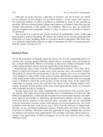
The input to our system is an MPEG or AVI video and a .wav file, containing the
music. As shown in Fig. 1, we start by segmenting both music and video, and then
analyze the features of each segment. To segment the music, we use novelty scoring
17 Automated Music Video Generation 387
Video clips
Music tracks
Video Segmentation
Velocity Extraction
Brightness Extraction
Video Analysis
Music Segmentation
Velocity Extraction
Brightness Extraction
Music Analysis
VSeg k
MSeg k
Domain normalizing
Matching
Subdivision
Render
Fig. 1 Overview of our music video generation system
[3], which detects temporal variation in the wave signal in the frequency domain. To
segment the video, we use contour shape matching [7], which finds extreme changes
of shape features between frames. Then we analyze each segment based on velocity
and brightness features.
Video Segmentation and Analysis
Synchronizing arbitrary lengths of video with the music is not a good way to pre-
serve the video-maker’s intent. Instead, we divide the video at discontinuities in the
flow, so as to generate segments that contain coherent information. Then we extract

features from each segment, which we use to match it with the music.
Segmentation by Contour Shape Matching
The similarity between two images can be simply measured as the difference be-
tween the colors at each pixel. But that is ineffective for a video only to detect short
388 J C. Yoon et al.
boundaries because the video usually contains movement and noise due to compres-
sion. Instead, we use contour shape matching [7], which is a well-known technique
for measuring the similarities between two shapes, on the assumption that one is a
distorted version of the other. Seven Hu-moments can be extracted by contour anal-
ysis, and these constitute a measure of the similarity between video frames which is
largely independent of camera and object movement.
Let V
i
.i D 1; :::; N/ be a sequence of N video frames. We convert V
i
to an
edge map F
i
using the Canny edge detector [2]. To avoid obtaining small contours
because of noise, we stabilize each frame of V
i
using Gaussian filtering [4]asa
preprocessing step. Then, we calculate the Hu-moments h
i
g
;.gD1; :::; 7/ from
the first three central moments [7]. Using these Hu-moments, we can measure the
similarity of the shapes in two video frames, V
i
and V

j
, as follows:
I
i;j
D
7
X
gD1
ˇ
ˇ
1=c
i
g
1=c
j
g
ˇ
ˇ
where
c
i
g
D sign

h
i
g

log
10

ˇ
ˇ
h
i
g
ˇ
ˇ
; (1)
and h
i
g
is invariant with translation, rotation and scaling [7]. I
i;j
is independent
of the movement of an object, but it changes when a new object enters the scene.
We therefore use large changes to I
i;j
to create the boundaries between segments.
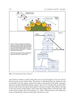
Figure 2a is a graphic representation of the similarity matrix I
i;j
.
Foote et al. [3] introduced a segmentation method that applies the radial sym-
metric kernel (RSK) to the similarity matrix (see Fig. 3). We apply the RSK to the
diagonal direction of our similarity matrix I
i;j
, which allows us to express the flow
discontinuity using the following equation:
Time
1st level 2nd level 3rd level
ba c

Fig. 2 Video segmentation using the similarity matrix: a is the full similarity matrix I
i;j
, b is the
reduced similarity matrix used to determine maximum kernel overlap region, and c is the result of
segmentation using different sizes of radial symmetric kernel
17 Automated Music Video Generation 389
0
0
0
Fig. 3 The form of a radially symmetric Gaussian kernel
EV.i/ D
ı
X
uDı
ı
X
vDı
RSK.u; v/  I
iCu;iCv
; (2)
where ı is the size of the RSK. Local maxima of EV.i/ are taken to be boundaries
of segments. We can control the segmentation level by changing the size of the
kernel: a large ı produces a coarse segmentation that ignores short variations in
flow, whereas a small ı produces a fine segmentation. Because the RSK is of size
ı and only covers the diagonal direction, we only need to calculate the maximum
kernel overlap region in the similarity matrix I
i;j
, as shown in Fig. 2b. Figure 2c
shows the result of for ı D32, 64 and 128, which are the values that we will use in
multi-level matching.

Video Feature Analysis
From the many possible features of a video, we choose velocity and brightness as the
basis for synchronization. We interpret velocity as a displacement over time derived
390 J C. Yoon et al.
from the camera or object movement, and brightness is a measure of the visual
impact of luminance in each frame. We will now show how we extract these features.
Because a video usually contains noise from the camera and the compression
technique, there is little value in comparing pixel values between frames, which is
what is done in the optical flow technique [17]. Instead, we use an edge map to track
object movements robustly. The edge map F
i
, described in the previous section can
be expected to outline. And the complexity of edge map, which is determined by
the number of edge points, can influence the velocity. Therefore, we can express the
velocity between frames as the sum of the movements of each edge-pixel. We define
a window 
x;y
.p; q/ of size ww, on edge-pixel point .x; y/ as its center, where p
and q are coordinates within that window. Then, we can compute the color distance
between windows in the i
th
and .i C 1/
th
frames as follows:
D
2
D
X
p;q2
i

x;y
.p;q/


i
x;y
.p; q/ 
iC1
.x;y/Cvec
i
x;y
.p; q/
Á
2
; (3)
where x and y are image coordinates. By minimizing the squared color distance,
we can determine the value of vec
i
x;y
. We avoid considering pixels which are not on
an edge, we assign a zero vector when F
i
.x; y/ D0. After finding all the moving
vectors in the edge map, we apply the local Lucas-Kanade optical flow technique
[14] to track the moving objects more precisely.
By summing the values of vec
i
x;y
, we can determine the velocity of the i
th

of the
video frames. However, this measure of velocity is not appropriate if a small area
outside the region of visual interest makes a large movement. In the next section,
we will introduce a method of video analysis based on the concept of significance.
Next, we determine the brightness of each frame of video using histogram
analysis [4]. First, we convert each video frame V
i
into a grayscale image. Then
we construct a histogram that partitions the grayscale values into ten levels. Using
this histogram, we can determine the brightness of the i
th
frame as follows:
V
i
bri
D
10
X
eD1
B.e/
2
B
mean
e
; (4)
where B.e/ is the number of pixels in the e
th
bucket and B
mean
e

is the representative
value of the e
th
bucket. Squaring B.e/ means that a contrasty image, such as a black-
and-white check pattern, will be classified as brighter than a uniform tone, even if
the mean brightness of all the pixels in each image is the same.
Detecting Significant Regions
The tracking technique, introduced in the previous section, is not much affected
by noise. However, an edge may be located outside the region of visual interest.
17 Automated Music Video Generation 391
This is likely to make the computed velocity deviate from a viewer’s perception
of the liveliness of the videos. An analysis of visual significance can extract the
region of interest more accurately. We therefore construct a significance map that
represents both spatial significance, which is the difference between neighboring
pixels in image space, and temporal significance, which measures of differences
over time.
We use the Gaussian distance introduced by Itti [10] as a measure of spatial sig-
nificance. Because this metric correlates with luminance [15], we must first convert
each video frame to the YUV color space. We can then calculate the Gaussian dis-
tance for each pixel, as follows:.
G
i
l;Á
.x; y/ D G
i
l
.x; y/  G
i
lCÁ
.x; y/; (5)

where G
l
is the l
th
level in the Gaussian pyramid, and x and y are image coordinates.
A significant point is one that has a large distance between its low-frequency and
high-frequency levels. In our experiment, we used the l D2 and Á D5.
The temporal significance of a pixel .x; y/ can be expressed as the difference in
its velocity between the i
th
and the .i C1/
th
frames, which we call its acceleration.
We can calculate the acceleration of a pixel from vec
i
x;y
, which is already required
for edge-map, as follows:
T
i
.x; y/ D N



vec
i
x;y
vec
iC1
x;y




; (6)
where N is a normalizing function which normalizes the acceleration so that it never
exceeds 1. We assume that a large acceleration brings a pixel to the attention of the
viewer. However, we have to consider the camera motion: if the camera is static, the
most important object in the scene is likely to be the one making the largest move-
ment; but if the camera is moving, it is likely to be chasing the most important object,
and then a static region is significant. We use the ITM method introduced by Lan
et al. [12] to extract the camera movement, with a 4-pixel threshold to estimate cam-
era shake. This threshold should relate to the size of the frame, which is 640 480
in this case. If the camera moves beyond that threshold, we use 1 T
i
.x; y/ rather
than T
i
.x; y/ as the measure of temporal significance.
Inspired by the focusing method introduced by Ma et al. [15], we then combine
the spatial and temporal significance maps to determine a center of attention that
should be in the center of the region of interest, as follows:
x
i
f
D
1
CM
n
X
xD1

m
X
yD1
G
i
.x; y/T
i
.x; y/x: (7)
y
i
f
D
1
CM
n
X
xD1
m
X
yD1
G
i
.x; y/T
i
.x; y/y;
392 J C. Yoon et al.
where
CM D
n
X

xD1
m
X
yD1
G
i
.x; y/T
i
.x; y/ (8)
and where x
i
f
and y
i
f
are the coordinates of the center of attention in the i
th
frame.
The true size of the significant region will be affected by motion and color distri-
bution in each video segment. But the noise in a home video prevents the calculation
of an accurate region boundary. So we fix the size of the region of interest at 1/4 of
the total image size. We denote the velocity vectors in the region of interest by vec
i
x;y
(see Fig. 4d), which those outside the region of interest are set to 0. We can then
calculate a representative velocity V
i
vel
, for the region of interest by summing the
pixel velocities as follows:

V
i
vel
D
n
X
xD1
m
X
yD1


vec
i
x;y


; (9)
where n m is the resolution of the video.
High velocity
Input video
ab
cd
Edge detection
Vector Map Final Vector Map
Low velocity
Fig. 4 Velocity analysis based on edge: a is a video segment; b is the result of edge detection;
c shows the magnitude of tracked vectors; and d shows the elimination of vectors located outside
the region of visual interest
17 Automated Music Video Generation 393

Home video usually contains some low-quality shots of static scenes or discon-
tinuous movements. We could filter out these passages automatically before starting
the segmentation process [8], but we actually use the whole video, because the
discontinuous nature of these low-quality passages means that they are likely to
be ignored during the matching step.
Music Segmentation and Analysis
To match the segmented video, the music must also be divided into segments. We
can use conventional signal analysis method to analyze and segment the music track.
Novelty Scoring
We use a similarity matrix to segment the music, which is analogous to our method
of video segmentation combined with novelty scoring, which is introduced by Foote
et al. [3] to detect temporal changes in the frequency domain of a signal. First, we
divide the music signal into windows of 1/30 second duration, which matches that
a video frame. Then we apply a fast Fourier transform to convert the signal in each
window into the frequency domain.
Let i index the windows in sequential order and let A
i
be a one-dimensional
vector that contains the amplitude of the signal in the i
th
window in the frequency
domain. Then the similarity of the i
th
and j
th
windows can be expressed as follows:
SM
i;j
D
A

i
A
j
kA
i
kkA
j
k
: (10)
The similarity matrix SM
i;j
can be used for novelty scoring by applying the same
radial symmetric kernel that we used for video segmentation as follows:
EA.i/ D
ı
X
uDı
ı
X
vDı
RSK.u; v/  SM
iCu;j Cv
; (11)
where ı D128. The extreme values of the novelty scoring EA.i / form the bound-
aries of the segmentation [3]. Figure 5 shows the similarity matrix and the corre-
sponding novelty score. As in the video segmentation, the size of the RSK kernel
determines the level of segmentation (see Fig. 5b). We will use this feature in the
multi-level matching that will follow in Section on “Matching Music and Video”.
394 J C. Yoon et al.
a

b
time
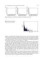
Fig. 5 Novelty scoring using the similarity matrix in the frequency domain: a is the similarity
matrix in the frequency domain; b the novelty scores obtained with different size of RSK
a
b
Fast Region
Slow Region
Fig. 6 a novelty scoring and b variability of RMS amplitude
Music Feature Analysis
The idea of novelty represents the variability of music (see Fig. 6a). We can also
introduce a concept of velocity for music, which is related to its beat. Many previ-
ous authors have tried to extract the beat from a wave signal [5, 18], but we avoid
confronting this problem. Instead we determine the velocity of each music segment
from the amplitude of the signal in the time domain.
We can sample the amplitude S
i
.u/ of a window i in the time domain, where u
is a sampling index. Then we can calculate a root mean square amplitude for that
window:
RMS
i
D
1
U
U
X
uD1
.S
i

.u//
2
; (12)
where U is the total number of samples in the window. Because the beat is usually
set by the percussion instruments, which dominate the amplitude of the signal, we
can estimate the velocity of the music from the RMS of the amplitude. If a music
segment has a slow beat, then the variability of the amplitude is likely to be relatively
17 Automated Music Video Generation 395
low; but if it has a fast beat then the amplitude is likely to be more variable. Using
this assumption, we extract the velocity as follows:
M
i
vel
DjRMS
i
RMS
i1
j: (13)
Figure 6a shows the result of novelty scoring and Fig. 6b shows the variability of
the RMS amplitude. We see that variability of the amplitude changes as the music
speeds up, but the novelty scoring remains roughly constant.
Popular music is often structured into a pattern, which might typically consist of
an intro, verse, and chorus, with distinct variations in amplitude and velocity. This
characteristic favors our approach.
Next, we extract the brightness feature using the well-known spectral centroid
[6]. The brightness of music is related to its timbre. A violin has a high spectral
centroid, but a tuba has a low spectral centroid. If A
i
.p/ is the amplitude of the
signal in the i

th
window in the frequency domain, and p is the frequency index, then
the spectral centroid can be calculated as follows:
M
i
bri
D
†p .A
i
.p//
2
†
.
A
i
.p/
/
2
: (14)
Matching Music and Video
In previous sections, we explained how to segment video and music and to extract
features. We can now assemble a synchronized music video by matching segments
based on three terms derived from the video and music features, and two terms
obtained from velocity histograms and segment lengths.
Because each segment of music and video has a different length, we need to
normalize the time domain. We first interpolate the features of each segment, espe-
cially velocity, brightness, and flow discontinuity, using a Hermite curve and then
normalize the magnitude of the video and music feature curves separately. The flow
discontinuity was calculated for segmentation and velocity and brightness features
were extracted both videos and music in previous sections. Using Hermite interpo-

lation, we can represent the k
th
video segment as a curve in a three-dimensional
feature space, V
k
.t/ D.cv
k
ext
.t/; cv
k
vel
.t/; cv
k
bri
.t//, ever the time interval [0, 1]. The
features of a music segment can be represented by a similar multidimensional curve,
M
k
.t/ D.cm
k
ext
.t/; cm
k
vel
.t/; cm
k
bri
.t//. We then compare the curves by sampling
them at the same parameters, using these matching terms:
– Extreme boundary matching Fc

1
.V
y
.t/; M
z
.t//.
The changes in Hu-moments EV.i/ in Eq. 2 determine discontinuities in the
video, which can then be matched with the discontinuities in the music found by
novelty scoring EA.i/ in Eq. 11. We interpolate these two features to create the
continuous functions cv
k
ext
.t/ and cm
k
ext
.t/, and then calculate the difference by
sampling them at the same value of the parameter t.
396 J C. Yoon et al.
– Velocity matching Fc
2
.V
y
.t/; M
z
.t//.
The velocity feature curves for video, cv
k
vel
.t/, and the music, cm
k

vel
.t/ can be
interpolated by V
i
vel
and M
i
vel
. These two curves can be matched to synchronize
the motion in the video with the beat of the music.
– Brightness matching Fc
3
.V
y
.t/; M
z
.t//.
The brightness feature curves for the video, cv
k
bri
.t/, and the music, cm
k
bri
.t/ can
be interpolated by V
i
bri
and M
i
bri

. These two curves can be matched to synchronize
the timbre of the music to the visual impact of the video.
Additionally, we used match the distribution of the velocity vector. We can gen-
erate a histogram VH
k
.b/ with K bins for the k
th
video segment using the video
velocity vector vec
x;y
. We also construct a histogram MH
k
.b/ of the amplitude of
the music in each segment, in the frequency domain A
k
. This expresses the timbre
of the music, which determines its mood. We define the cost of matching each pair
of histogram as follows:
Hc.y; z/ D
K
X
bD1
Â
VH
y
.b/
N
y

MH

z
.b/
N
z
Ã
2
; (15)
where y and z are the indexes of a segment, and N
y
and N
z
are the sum of the car-
dinality of the video and music histograms. This associates low-timbre music with
near-static video, and high-timbre music with video that contains bold movements.
Finally, the durations of video and music should be compared to avoid the need for
excessive time-warping. We therefore use the difference of duration between the
music and video segments as the final matching term, Dc.y; z/. Because the range
of Fc
i
.V
y
.t/; M
z
.t// and Hc.y; z/ are [0,1], we normalize the Dc.y; z/ by using
the maximum difference of duration.
We can now combine the five matching terms into the following cost function:
Cost
y;z
D
3

X
iD1
w
i
Fc
i
.V
y
.t/; M
z
.t// C w
4
Hc.y; z/ C w
5
Dc.y; z/; (16)
where y and z are the indexes of a segment, and w
i
is the weight applied to each
matching terms. The weights control the importance given to each matching term.
In particular, w
5
, which is the weight applied to segment length matching, can be
used to control the dynamics of the music video. A low value of w
5
allows more
time-warping.
We are now able to generate a music video by calculating Cost
y;z
for all pairs
of video and music segments, and then selecting the video segment which matches

each music segment at minimum cost. We then apply time-warping to each video
segment so that its length is exactly the same as that of the corresponding music
segment. A degree of interactivity is provided by allowing the user to remove any
displeasing pair of music and video segments, and then regenerate the video. This
facility can be used to eliminate repeated video segments. It can also be extended,
so that the user is presented with a list of acceptable matches form which to choose
a pair.
17 Automated Music Video Generation 397
We also set a cost threshold to avoid low-quality matches. If a music segment
cannot be matched with a cost lower than the threshold, then we subdivide that
segment by reducing the value of ı in the RSK. Then we look for a new match to
each of the subdivided music segments. Matching and subdivision can be recursively
applied to increase the synchronization of the music video; but we limit this process
to three levels to avoid the possibility of runaway subdivision.
Experimental Results
By trial and error, we selected (1, 1, 0.5, 0.5, 0.7) for the weight vector in Eq. 16,
set K D32 in Eq. 15, and set the subdivision threshold to 0:3 mean.Cost
y;z
/.
For an initial test, we made a 39-min video (Video 1) containing sequences
with different amount of movement and levels of luminance (see Fig. 7). We also
composed 1 min and 40 s of music (Music 1), with varying timbre and beat. In
the initial segmentation step, the music was divided into 11 segments. In the sub-
sequent matching step, the music was subdivided into 19 segments to improve
synchronization.
We then went on to perform more realistic experiments with three short films and
one home video (Videos 2, 3, 4 and 5: see Fig. 8), and three more pieces of music
which we composed. From this material we created three sets of five music videos.
The first set was made using Pinnacle Studio 11 [1]; the second set was made using
Fig. 7 Video filmed by the authors

398 J C. Yoon et al.
Video 2
ab
cd
Video 3
Video 4 Video 5
Fig. 8 Example videos: a Short film “Someday”, directed by Dae-Hyun Kim, 2006; b Short
film “Cloud”, directed by Dong-Chan Kim; c Short film “Father”, directed by Hyun-Wook Moon;
d Amateurs home video “Wedding”
Foote’s method [3]; and the third was produced by our system. The resulting videos
can all be downloaded from URL.
1
We showed the original videos to 21 adults who had no prior knowledge of this
research. Then we showed the three sets of music videos to the same audience, and
asked them to score each video, giving marks for synchronization (velocity, bright-
ness, boundary and mood), dynamics (dynamics), and the similarity to the original
video (similarity), meaning the extent to which the original story-line is presented.
The ‘mood’ term is related to the distribution of the velocity vector and ‘dynamics’
term is related to the extent to which the lengths of video segments are changed by
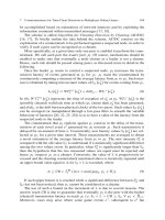
time-warping. Each of the six terms was given a score out of ten. Figure 9 shows
that our system obtained better than Pinnacle Studio as Foote’s methods on five out
of the six terms. Since our method currently makes no attempt to preserve the orig-
inal orders of the video segments, it is not surprising that the result for ‘similarity’
were more ambiguous.
Table 1 shows the computation time required to analyze the video and music. We
naturally expect the video to take much longer to process than the music, because
of its higher dimensionality.
1
/>17 Automated Music Video Generation 399
Velocity Brightness

Mood
Dynamics Boundary Simiarity
Pinnacle studio Foote's method Our method
0
1
2
3
4
5
6
7
8
9
Fig. 9 User evaluation results
Table 1 Computation times
for segmentation and analysis
of music and video
Media Length Segmentation Velocity Brightness
Video 1 30 min 50 min 84 min 3 min
Video 2 23 min 44 min 75 min 2.5 min
Video 3 17 min 39 min 69 min 2.1 min
Video 4 25 min 46 min 79 min 2.6 min
Video 5 45 min 77 min 109 min 4.1 min
Music 1 100 s 7.2 s 4.2 s 2.1 s
Table 2 A visual count of
the numbers of shots in each
videos, and the number of
segments generated using
different values of ı in
the RSK

Visually
counted
num. of
Media shots ı D128 ı D 64 ı D 32
Video 1 44 49 63 98
Video 2 34 41 67 142
Video 3 36 50 57 92
Video 4 43 59 71 102
Video 5 79 92 132 179
Table 2 shows how the number of video segments was affected by the value
of ı in the RSK. We also assessed the number of distinct shots in each video by
inspection. This visual count tallies quite well with the results when ı D128.By
reducing ı to 32, the number of distinct shots are approximately doubled.
Table 3 shows computation times for matching the music and video. Because the
matching is takes much less time than analysis, we stored the all the feature curves
for both video and music to speed up the calculations.
400 J C. Yoon et al.
Table 3 Computation times
for matching Music 1 to the
five videos
Media Time (s)
Video 1 6:41
Video 2 8:72
Video 3 6:22
Video 4 7:48
Video 5 10:01
Conclusion
We have produced an automatic method for generating music videos that preserves
the flow of video segments more effectively than previous approaches. Instead of
trying to synchronize arbitrary regions of video with the music, we use multi-level

segment matching to preserve more of the coherence of the original videos. Provided
with an appropriate interface to simplify selection of the weight terms, this system
would allow music video to be made with very little skill.
The synchronization of segments by our system could be improved. Although
each segment is matched in terms of features, it is possible for points of discordancy
between music and video to remain within a segment. We could increase the level
of synchronization by applying time-warping within each segment using features
[13]. Another area of concern is the time required to analyze the video, and we are
working on a more efficient algorithm.
Many home videos have a weak story-line, so that the original sequence of the
video may not be important. But this will not be true for all videos, and so we need
to look for ways of preserving the story-line, which might involve a degree of user
annotation.
Acknowledgements This research is accomplished as the result of the promotion project for cul-
ture contents technology research center supported by Korea Culture & Content Agency (KOCCA).
References
1. Avid Technology Inc (2007) User guide for pinnacle studio 11. Avid Technology Inc,
Tewksbury
2. Canny J (1986) A computational approach to edge detection. IEEE Trans Pattern Anal Mach
Intell 8(6):679–698
3. Foote J, Cooper M, Girgensohn A (2002) Creating music videos using automatic media anal-
ysis. In: Proceedings of ACM multimedia. ACM, New York, pp 553–560
4. Gose E, Johnsonbaugh R, Jost S (1996) Pattern recognition and image analysis. Prentice Hall,
Englewood Cliffs
5. Goto M (2001) An audio-based real-time beat tracking system for music with or without drum-
sounds. J New Music Res 30(2):159–171
6. Helmholtz HL (1954) On the sensation of tone as a physiological basis for the theory of music.
Dover (translation of original text 1877)
17 Automated Music Video Generation 401
7. Hu M (1963) Visual pattern recognition by moment invariants. IRE Trans Inf Theo 8(2):

179–187
8. Hua XS, Lu L, Zhang HJ (2003) Ave—automated home video editing. In: Proceedings of
ACM multimedia. ACM, New York, pp 490–497
9. Hua XS, Lu L, Zhang HJ (2004) Automatic music video generation based on temporal pattern
analysis. In: 12th ACM international conference on multimedia. ACM, New York, pp 472–475
10. Itti L, Koch C, Niebur E (1998) A model of saliency-based visual attention for rapid scene
analysis. IEEE Trans Pattern Anal Mach Intell 20(11):1254–1259
11. Jehan T, Lew M, Vaucelle C (2003) Cati dance: self-edited, self-synchronized music video.
In: SIGGRAPH conference abstracts and applications. SIGGRAPH, Sydney, pp 27–31
12. Lan DJ, Ma YF, Zhang HJ (2003) A novel motion-based representation for video mining. In:
Proceedings of the IEEE international conference on multimedia and expo. IEEE, Piscataway,
pp 6–9
13. Lee HC, Lee IK (2005) Automatic synchronization of background music and motion in com-
puter animation. In: Proceedings of eurographics 2005, Dublin, 29 August–2 September 2005,
pp 353–362
14. Lucas B, Kanade T (1981) An iterative image registration technique with an application to
stereo vision. In: Proceedings of 7th international joint conference on artificial intelligence
(IJCAI), Vancouver, August 1981, pp 674–679
15. Ma YF, Zhang HJ (2003) Contrast-based image attention analysis by using fuzzy growing. In:
Proceedings of the 11th ACM international conference on multimedia. ACM, New York, pp
374–381
16. Mulhem P, Kankanhalli M, Hasan H, Ji Y (2003) Pivot vector space approach for audio-video
mixing. IEEE Multimed 10:28–40
17. Murat Tekalp A (1995) Digital video processing. Prentice Hall, Englewood Cliffs
18. Scheirer ED (1998) Tempo and beat analysis of acoustic musical signals. J Acoust Soc Am
103(1):588–601
Part III
DIGITAL VISUAL MEDIA
Chapter 18
Real-Time Content Filtering for Live Broadcasts

in TV Terminals
Yong Man Ro and Sung Ho Jin
Introduction
The growth of digital broadcasting has lead to the emergence and wide spread
distribution of TV terminals that are equipped with set-top boxes (STB) and per-
sonal video recorders (PVR). With increasing number of broadcasting channels and
broadcasting services becoming more personalized, today’s TV terminal requires
more complex structures and functions such as picture-in-picture, time-shift play,
channel recording, etc. The increasing number of channels also complicates the ef-
forts of TV viewers in finding their favorite broadcasts quickly and efficiently. In
addition, obtaining meaningful scenes from live broadcasts becomes more difficult
as the metadata describing the broadcasts is not available [1]. In fact, most live
broadcasts cannot afford to provide related metadata as it must be prepared before
the broadcast is aired.
Until now, many scene detection and content-indexing techniques have been
applied to video archiving systems for video summarization, video segmentation,
content management, and metadata authoring of broadcasts [2–7]. Some of them
have been applied in STB or PVR after recording entire broadcasts [8–10]. Cur-
rent broadcasting systems provide simple program guiding services with electronic
program guides, but do not provide meaningful scene searching for live broadcasts
[11, 12]. In order to provide a user-customized watching environment in digital
broadcasting, meaningful scene search in real-time is required in the TV termi-
nal. N. Dimitrova et al. [13], studied video analysis algorithms and architecture for
abstracted video representation in consumer domain applications and developed a
commercial tool for skipping through the detection of black frames and changes in
activity [14]. Our work, however, focuses on establishing a system that enables the
indexing and analyzing of live broadcasts at the content-level.
The goal of this chapter is to develop a service that provides content-level infor-
mation within the limited capacity of the TV terminal. For example, a TV viewer
Y. M . Ro (


) and S.H. Jin
IVY Lab, Information and Communications University, Daejon, Korea
e-mail:
B. Furht (ed.), Handbook of Multimedia for Digital Entertainment and Arts,
DOI 10.1007/978-0-387-89024-1 18,
c
Springer Science+Business Media, LLC 2009
405
406 Y.M. Ro and S.H. Jin
watches his/her favorite broadcasts (e.g., a drama or sitcom) on one channel, while
the other channels broadcast other programs (e.g., the final round of a soccer game)
that also contain scenes of interest to the viewer (e.g., shooting or goal scenes).
To locate these scenes of interest on other channels, a real-time filtering technique,
which recognizes and extracts meaningful contents of the live broadcast, should be
embedded in the TV terminal. In this chapter, a new real-time content filtering sys-
tem for a multi-channel TV terminal is proposed. The system structure and filtering
algorithm have been designed and verified. The system’s filtering requirements such
as, the number of available input channels, the frame sampling rate, and buffer size
were analyzed based on queueing theory, and filtering performance was calculated
so as to maintain a stable filtering system.
The chapter is organized as follows. We first give an overview of the proposed
system and general filtering procedure in Section II. Section III shows the analysis
of filtering system based on the queue model. Section IV presents experiments in
which soccer videos were tested in the proposed system and shows the experimental
results of five soccer videos. Realization of the proposed system is discussed in
Section V, and concluding remarks are drawn in Section VI.
Real-time Content Filtering System
In this section, we explain the structure of a real-time broadcasting content filtering
system in a TV terminal. In addition, a filtering algorithm for multiple broadcasts

is proposed, which is simplified for real-time processing and shows a promising
filtering performance. Typical processing of face-name association is as follows:
Filtering System Structure
The system structure of a TV terminal for the real-time content filtering function
is illustrated in Fig. 1. In this work, the terminal is assumed to have more than two
TV tuners. One of the tuners receives a broadcast stream from the main channel to
be watched, and the rest receive streams from the selected channels to be filtered. It
is assumed that the TV viewer is interested in the selected channels as well as the
main channel.
As shown in Fig. 1, a selected broadcast from the main channel is conveyed to
the display unit after passing through demux, buffer, decoder, and synchronizer. In
the content filtering part, meaningful scenes are extracted from input broadcasts and
filtered results are sent to the display unit. The receiver components, i.e. the demux
and the decoder, before the content filtering part, are supposed to be able to support
the decoding of multi-streams.
18 Real-Time Content Filtering for Live Broadcasts in TV Terminals 407
Fig. 1 System structure of TV terminal for real-time content filtering
The number of allowable input channels required to guarantee real-time filtering
depends on frame sampling rate, buffer condition, etc. (these are discussed in detail
in Section III).
Real-Time Content Filtering Algorithm
In the terminal of Fig. 1, the content filtering part monitors channels and selects
meaningful scenes based on the TV viewer’s preference. As soon as the terminal
finds the selected scenes, that is, the viewer’s desired scenes filtered from his/her
channels referred to as “scenes of interest,” it notifies this fact by means of the chan-
nel change or channel interrupt function. The picture-in-picture function currently
available in TVs is useful for displaying the filtering results.
To filter the content of the broadcast, sampling and processing of multiple in-
put broadcasts should be performed without delay. Figure 2 shows the proposed
filtering algorithm through which a TV viewer not only watches the broadcast of

the main channel, but also obtains meaningful scenes of broadcasting content from
other channels. The procedure of the filtering process is as follows.
Step 1: A viewer logs on to a user terminal.
Step 2: After turning on the real-time filtering function, the TV viewer chooses
filtering options such as scenes of interest. Simultaneously, the viewer’s prefer-
ence database is updated with new information on the selected scenes.
Step 3: In a TV decoder, the filtering part in Fig. 1 receives video streams of
broadcasts and acquires frames by sampling in regular intervals.
Step 4: The sampled frames are queued in a buffer followed by feature extraction.
This step is repeated during the filtering process.
Step 5: Image and video features such as color, edge, and motion from the sam-
pled frame are extracted to represent the spatial information of the frame.
408 Y.M. Ro and S.H. Jin
Fig. 2 Proposed real-time broadcasting content filtering algorithm
Step 6: The view type of the input frame is decided according to visual features.
After completing this step, a new frame is fetched for the next feature extraction.
Step 7: Desired scenes are detected by the pattern of temporal frame sequences
such as view type transition or continuity.
Step 8: Finally, the filtering process is concluded with the matched filtering result.
In Step 5, the feature extraction time depends on the content characteristics of the
input frame. Broadcasting video consists of various types of frames represented by
various features (e.g., color, edge. etc.). Therefore, we need to avoid the overflow
problem at the buffer caused by the feature extraction time.
18 Real-Time Content Filtering for Live Broadcasts in TV Terminals 409
Filtering System Analysis
Since real-time filtering should be performed within a limited time, frame sampling
rate to filter, buffer size to input frames, and the number of allowable input channels,
should be suitably determined to achieve real-time processing.
Modeling of a Filtering System
In Fig. 2, the inputs of the filtering part are the sampled frames from the decoder in

regular sampling rate. The frames waiting for filtering should be buffered because
the filtering processing time is irregular. Thus, filtering can be modeled by queueing
theory. Figure 3 illustrates the queue model for the proposed filtering system for N
input channels. The frames sampled from the input channels are new customers in
the buffer and the filtering process is a server for customers. Before being fetched
to the server, the frames wait for their orders in the buffer. In the figure, f is the
sampling rate which denotes the number of sampled frames per second from one
channel.
As shown in the Fig.3, frames are acquired by sampling periodically arriving
video streams at the buffer. After filtering a frame, the next frame in the buffer
is taken out irregularly in the order of its arrival at the buffer. Note that the filtering
time for the video frame is irregular and depends on the content characteristics of
the frame.
The proposed filtering system is designed as a queue model with the following
characteristics: 1) arrival pattern of new customers into the queue, 2) service pattern
of servers, 3) the number of service channels, 4) system capacity, 5) number of
service stages, and 6) the queueing policy [15–18].
Fig. 3 Queue model of content filtering for multiple channels
410 Y.M. Ro and S.H. Jin
Fig. 4 Queueing process for successive frames
First, we consider the distributions of the buffer in terms of inter-arrival time
between sampled frames and service time between filtered frames. In Fig. 4,let
T(n) represent the inter-arrival time between nth and .n C 1/st customers (sampled
frames), and S(n) represent the service time of the nth customer. As seen in Fig. 3,
the inter-arrival time is determined by a regular sampling rate, i.e. the inter-arrival
time is constant. We can see that the probability distribution describing the time
between successive frame arrivals is deterministic.
Given that the view types of the frames in a queue are statistically independent,
follow a counting process, and have different service times (filtering times), we as-
sume that the number of filtering occurrences within a certain time interval becomes

a Poisson random variable. Then, the probability distribution of the service time is
an exponential distribution. A D/M/1 queue model can be applied to model the pro-
posed filtering system, which covers constant inter-arrivals to a single-server queue
with exponential service time distribution, unlimited capacity and FCFS (first come,
first served) queueing discipline.
However, the D/M/1 model may cause buffer overflow and decrease filtering
performance by frame loss when the buffer is feed with frames of the same type, a
situation which has the longest processing time. Thus, if the service (filtering) time
of one frame is longer than the inter-arrival time, the waiting frames pile within the
buffer. Therefore, filtering policies such as frame skipping or dropping of sampling
rate are required.
To find a sufficient condition in which the filtering system remains stable, the
worst case is considered. We assume the worst case is one in which the buffer is
occupied by frames with the longest filtering time sampled from multiple channels.
The pattern of filtering times for successive similar frames is constant. Therefore,
the two probability patterns can be established as deterministic distributions.
In the above model, the number of filtering processes and the length of buffer
are 1 and 1(I don’t understand why it is 1 and 1?), respectively; and the queueing
discipline for filtering is FCFS. Thus, the stable filtering system in which the worst
case is considered can be explained as a D/D/1 queue model in a steady state.
Requirements of Stable Real-Time Filtering.