High Cycle Fatigue: A Mechanics of Materials Perspective part 65 potx

626 Appendix I
from Hawkyard et al. [12] and are assumed to decrease linearly from 5MPa
√
mto
225 MPa
√
matR=07 and maintain values of 5 and 225 MPa
√
matR<0 and R>07,
respectively. The stress intensity factor solution of Raju and Newman [13] for surface
cracked smooth bars is utilized, and assumptions are made concerning the geometry of
the crack such that the stress intensity factor may be approximated as
K =

a
163

1+
a
D

(I.5)
where a is the crack depth and D is the diameter of the bar. Due to the presence of the
notch, the applied stress is multiplied by a K
T
of 2 in order to determine K
HCF
, K
LCF
,
a

crit
, a
gHCF
, and a
gLCF
. This is an appropriate assumption when the crack is very short.
However, as the crack extends out of the notch, it has been shown that the crack growth
rate will approach that for K
T
=1 and a crack depth equaling the total depth of the crack
and notch [14]. These assumptions using K
T
are conservative and will cause the model
to underestimate the crack propagation life. However, under the conditions of interest,
the propagation life is a small percentage of the total life.
NUMERICAL RESULTS
The numerical algorithm has been implemented on a personal computer and operates in
one of two modes. In the first mode, the user specifies 
a
, 
m
, and n, and the total life
corresponding to 10
7
HCF cycles is calculated in terms of CCF load blocks, N. In the
second mode, the user specifies 
m
, N, and n, and an iterative algorithm is invoked to
determine 
a

such that the calculated value of N is within a specified tolerance of the
requested value of N. Solution time increases with increasing N and increasing fraction
of total life spent in crack propagation, especially when the crack is actively growing in
both HCF and LCF cycles. For the most computationally intensive cases considered, the
solution took no more than one to two minutes on a 100-MHz personal computer.
Correlation with experiment
A limited number of HCF–LCF tests on notched bars were conducted by Guedou and
Rongvaux [9]. Ti-6Al-4V bars were cycled at room temperature with n =1800 HCF cycles
per CCF load block and R
HCF
=085. The resulting initiation lives are shown along with
those for LCF-only tests in Figure I.4. All results are plotted as a function of maximum
stress (
m
+
a
). A power law fit to the LCF-only initiation data is also shown. This fit
was used to define the S–N curve shown in Figure I.3 which, in turn, defines the constants
for use in the modified Goodman equation over intermediate values of alternating stress
range. Predictions for the HCF–LCF initiation life using Equation (I.2) are also shown
Appendix I 627
10
2
10
3
10
4
600
700
800

900
1000
LCF only (Experimental)
LCF only (Correlation)
CCF (Experimental)
CCF (Predicted with endurance limit)
CCF (Predicted with no endurance limit)
LCF cycles (or CCF load blocks) to initiation
Maximum stress (MPa)
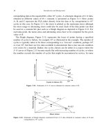
Figure I.4. Comparison of predicted and measured LCF and CCF initiation life for Ti-6-4 [9] with R
HCF
=085
and n=1800.
for both scenarios: 
end
=300 MPa and 
end
=0. As expected, the predictions are
identical for cases in which 
HCF
> 300MPa. At high values of maximum stress, both
assumptions overestimate the detrimental effect of HCF cycles on the initiation life. At
lower maximum stress levels, the best correlation is found when 
end
=0.
Figure I.5 shows a similar comparison of experimentally inferred and numerically
predicted crack propagation lives for the LCF-only and HCF–LCF tests of Guedou and
Rongvaux [9]. The numerical predictions underestimate the propagation lives of the LCF-
only tests. This is expected, since K
T

at the crack tip has been taken as two over the
entire life of the crack. As discussed earlier, this is a conservative assumption which is
expected to underestimate the propagation life. Predicted values for the HCF–LCF tests
are, of course, the same under either endurance limit assumption. The drastic change in
slope is unrelated to that of the finite endurance limit assumption shown in Figure I.4. In
Figure I.5, it is a function of K
th
. The number next to each predicted point corresponds
to the fraction of propagation life over which the crack does not grow in HCF. (The
crack grows in CCF during the remainder of the propagation life.) The four highest
stress predictions begin growing in CCF immediately upon crack initiation (Path 3 in
Figure I.2). In these cases, crack propagation life is underestimated by approximately
an order of magnitude. At lower values of maximum stress (and constant R
HCF
), K
HCF
is initially below K
th
at crack initiation and the crack must propagate for a period in
LCF-only before CCF crack growth can occur (Path 6 in Figure I.2.). Better correlation
with experiment is obtained at lower stresses, possibly indicating that the values of K
th
628 Appendix I
10
1
10
2
10
3
600

700
800
900
1000
LCF only (Experimental)
LCF only (Predicted)
CCF (Experimental)
CCF (Predicted)
Propagation life (LCF cycles or CCF load blocks)
Maximum stress (MPa)
0.00
0.00
0.00
0.00
0.57
0.88
0.92
0.93
Figure I.5. Comparison of predicted and measured LCF and CCF crack propagation life for Ti-6-4 [9] with
R
HCF
=085 and n=1800.
as a function of R used here are lower than those in the material tested. Guedou and
Rongvaux [9] estimate K
th
=3MPa
√
matR=085, whereas K
th
=225 at R=085

has been used here.
Finally, Figure I.6 shows the correlation between the experimentally measured and
predicted vales of total life. The total life is dominated by the initiation life. Thus,
the assumption of no endurance limit gives better correlation with the total life. The
assumptions concerning the K
T
at the crack tip during crack propagation have little effect
on the correlation with total life. Unless otherwise noted, subsequent results are calculated
under the assumption of no endurance limit.
Effect of LCF on HCF capability
Figure I.7 shows the computed values of allowable 
a
as a function of 
m
for failure in
10
7
HCF cycles (plus one LCF cycle representing the initial loading to a peak stress of

a
+
m
.) Line 1 indicates the alternating and mean stress combinations which will cause
initiation in 10
7
HCF cycles with no superimposed LCF cycles N =1. If the number of
cycles to initiation is increased from 10
7
to 10
8

, the line moves down as shown. Another
curve (line 2) is drawn to indicate the stress states above which a crack will propagate
under HCF based on an initiation crack size (50 m here) and the assumed value of K
th
as a function of R. At low values of mean stress, this line has a slope which increases
significantly and follows a line along which 
a
+
m
=constant. This value of maximum
Appendix I 629
10
2
10
3
10
4
600
700
800
900
1000
LCF only (Experimental)
LCF only (Predicted)
CCF (Experimental)
CCF (Predicted with no endurance limit)
CCF (Predicted with endurance limit)
Total Life (LCF cycles or CCF load blocks)
Maximum stress (MPa)
Figure I.6. Comparison of predicted and measured LCF and CCF total life for Ti-6-4 [9] with R

HCF
=085
and n=1800.
0
50
100
150
200
250
0 200 400 600 800 1000 1200
Alternating stress (MPa)
Mean stress (MPa)
LINE 3: N
I,LCF
= 1
LINE 1: N
I,HCF
= 10
7
LINE 2: ΔK
th,HCF
R = 0
R = 0.7
N
I,HCF
= 10
8
LINE 4: ΔK
th,LCF
Figure I.7. Haigh diagram as predicted by analysis showing underlying mechanisms which govern the shape

of the solution curve.
630 Appendix I
stress corresponds to K
HCF
=K
th
at the initiating crack length. Note that in this low
mean stress region, corresponding to negative R, the crack can initiate in less than 10
7
HCF cycles at stress states above line 1 but will never propagate if the stress state is
below line 2. Conversely, there is a region bounded by 200 <
m
< 600MPa where the
crack will not initiate (below line 1), yet a 50-m crack could propagate (above line 2)
based on the assumptions in this analysis. If the numerical assumptions are correct, this
would imply that within this range of mean stresses, which is in a “safe” design space
for initiation based on an initiation criterion represented in a Haigh diagram, the material
is intolerant to small amounts of damage. For initial defects or service induced damage
such as FOD equivalent to a crack of 50 m or greater, that damage would grow and
eventually cause failure under HCF loading. This could occur, even though the stress
states in this region indicate that cracks would not initiate under either LCF or HCF.
Following the same series of assumptions, additional curves can be drawn for the
boundaries below which LCF cycles will not cause initiation in a specified number, N ,
of cycles, or below which a 50-m crack will not propagate. The initiation curve for
N =1 LCF cycle is shown as line 3 in Figure I.7 and represents 
a
+
m
=
ult

. Any stress
state above or to the right of this line will cause tensile failure on the first cycle. Finally,
above and to the right of line 4, crack growth will occur under LCF loading once a crack
initiates. Note that line 4 coincides with line 2 at low values of 
m
, above which HCF
crack growth will occur (for a 50-m crack). This is due to the assumption that the crack
is closed at  =0 so that for R
HCF
< 0, K
LCF
=K
HCF
. Under the assumptions of this
analysis, the region where failure can occur due to either HCF or LCF is above the heavy
line in Figure I.7.
The safe design space defined for N =1 in Figure I.7 can be determined for other
values of N. Figure I.8 shows solutions for various values of N and n where Nn=10
7
.
As N increases, the allowable alternating stress decreases at higher values of mean stress.
As expected, a finite number of LCF cycles reduces the maximum mean stress that may
safely be applied to the structure. Comparison of Figures I.3 and I.8 indicates that the
limiting value of mean stress for a given value of N corresponds to the allowable stress
range for a specified value of N in Figure I.3.
Parametric studies
Inherent in the previous analyses were several assumptions concerning the behavior of
the material. Among these were the variation in K
th
with R and the form of the initiation

damage relationship. In each case, alternate assumptions can be used and lead to different
results. Here, we consider the sensitivity of the results to such changes.
First, consider the form of the K
th
versus R behavior. Experimentally measured
values of K
th
as a function of R are shown in Figure I.9 [12] for Ti-6-4. Two fits
to the experimental data are also shown. A piecewise linear fit is shown which can be
Appendix I 631
0
50
100
150
200
250
0 200 400 600 800 1000 1200
N

=

10
0
, n

=

10
7
N

=

10
2
, n

=

10
5
N

=

10
3
, n

=

10
4
N

=

10
4
, n

=

10
3
N

=

10
5
, n

=

10
2
Alternating stress (MPa)
Mean stress (MPa)
R = 0
R = 0.5
R = 0.818
R = 0.667
N = 1
(Tensile overload)
N = 1 (n = 10
7
)
Initiation line
Figure I.8. Effect of number of superimposed LCF cycles on the HCF capability of Ti-6-4 as estimated by

analysis.
0
1
2
3
4
5
6
0 0.2 0.4 0.6 0.8 1
Closure model
CTOD model (Taylor, 1988)
Experimental (Hawkyard et al., 1996)
Δ
K
th

(MPa √m)
R
Figure I.9. Comparison of CTOD-based and closure-based K
th
vs R models with experimental data
on Ti-6-4 [12].
632 Appendix I
rationalized through closure arguments and is incorporated into the previous analyses. As
an alternative, K
th
may be defined as
K
th
=K

tho

1−R
1+R

05
(I.6)
which is based on cyclic crack-tip opening displacement (CTOD) arguments [15]. In each
case, a least squares approach has been used to obtain an optimal fit to the experimental
data. Although in this material, the closure-based approach clearly correlates better with
experiment, data obtained on other materials have been shown to correlate well with the
CTOD approach [15, 16].
Figure I.10 indicates how the different variations in K
th
with R affect the form of the
solution. The dashed lines indicate the magnitude of alternating stress required to cause
crack propagation in a 50 -m-deep crack using K
th
variation based on both closure
and CTOD models. Differences in the solution for allowable 
a
versus 
m
are significant
and are particularly noticeable at high R. Thus, the variation in K
th
at high R appears
to be important in predicting HCF life as a function of mean stress. Figure I.11 repeats
the results shown in Figure I.8 which show the allowable 
a

versus 
m
for various
combinations of HCF and superimposed LCF. Here, however, predictions are made using
both CTOD and closure-based K
th
R values. Note that while the differences between
the methods are significant for small values of N at high mean stress, when N becomes
sufficient to cause reductions in the allowable alternating stress (versus pure HCF), the
results become relatively insensitive to the K
th
model in use.
0
50
100
150
0 200 400 600 800 1000 1200
Alternating stress (MPa)
Mean stress (MPa)
ΔK
th
by
CTOD theory
Initiation life
= 10
7
ΔK
th
by
closure theory

(line 2 from Fig. 7)
Solution
(closure ΔK
th
)
Solution
(CTOD ΔτK
th
)
N = 1
(Tensile overload)
Figure I.10. Effect of K
th
vs R model on the HCF-only Haigh diagram as predicted by analysis.
Appendix I 633
0
50
100
150
0 200 400 600 800 1000 1200
N = 1
N = 100
N = 1,000
N = 10,000
N = 1
N = 100
N = 1000
N = 10,000
Alternating stress (MPa)
Mean stress (MPa)

R = 0 R = 0.5
R = 0.905
R = 0.818
R = 0.967
ΔK
th
by closure theory
ΔK
th
by CTOD theory
Figure I.11. Effect of K
th
vs R model on the CCF Haigh diagram as predicted by analysis.
0
50
100
150
200
250
0 200 400 600 800 1000 1200
N = 1
N = 10,000
N = 1
N = 10,000
Alternating stress (MPa)
Mean stress (MPa)
R = 0 R = 0.5
R
= 0.905
R

= 0.818
R
= 0.667
N = 1 (n = 10
7
)
Initiation line
(No endurance limit
)
2 σ
end
= 0 MPa
2 σ
end
= 300 MPa
N = 1 (n = 10
7
)
Initiation line
(finite endurance limit
)
Figure I.12. Effect of endurance limit assumption on the HCF-only and CCF (N = 10000) Haigh diagrams
as predicted by analysis.
In Figure I.12, Haigh diagrams are shown for two different initiation phase assump-
tions: (a) the case of “no endurance limit” such that HCF cycles of infinitesimal stress
amplitude cause finite damage (as incorporated in the previous analyses) and (b) the
634 Appendix I
case of 
end
=300MPa. Results are shown for N =1 and 10,000. The presence of

an endurance limit effectively raises the initiation line (line 1 in Figure I.7). Note that
the intersection of the solution for 
end
= 300MPa and the R = 0 line corresponds to
half the endurance limit stress range which again matches the 10
7
initiation life point in
Figure I.3.
CLOSURE
Discussion
The numerical results presented here are based on simple models of crack initiation and
propagation. Many potentially important phenomena are neglected such as the possi-
ble non-linear accumulation of initiation damage, the effect of previous cycling on the
instantaneous endurance limit, acceleration in the HCF crack growth rate due to periodic
underloads (LCF cycles), reduction in K
th
as a function of the number of LCF cycles,
small crack effects, hold time effects on LCF cycles, and many more. Therefore, these
results must be viewed as preliminary, giving only a qualitative indication of how LCF
and HCF cycling interact to reduce overall life. Although simple, the method satisfacto-
rily predicts the effects of combined HCF–LCF loading (see, e.g. Figure I.5) despite the
limited amount of experimental data available for calibration. Additional experimental
results should allow for better calibration and will pave the way for incorporation and
assessment of many of the above phenomena.
Although the Goodman assumption is used in accounting for mean stress effects in crack
initiation, the resulting Haigh diagram obtained differs from the Goodman assumption
for total life in two regions as shown, for example, in Figure I.7. At very low mean
stress, the predicted response curve follows lines 2 and 4, and is significantly steeper
than that displayed by the Haigh diagram. At high mean stress, the allowable alternating
stress follows line 2 and remains constant up to very high mean stress. In both high and

low mean stress cases, the differences between the predicted response and the expected
Goodman-type response (i.e. a straight line) are due to regions in the Haigh diagram in
which a crack is predicted to initiate but not grow. For the experimental data considered
here, this phenomenon may be due to the small crack size considered (a
i
=50 m) which
may exhibit increased crack growth rates due to small crack effects. Such effects are
not considered in this analysis. If a longer initial crack size were considered, both lines
2 and 4 in Figure I.5 would move down and to the left resulting in a solution curve
which looks more like the Haigh diagram. Note also that considering a K
th
versus R
curve for which K
th
⇒ 0asR ⇒ 1 also results in a solution curve which approaches
the Goodman assumption as shown in Figure I.10. Interestingly, the solution curve
shown in Figure I.7 is similar in form to the experimental results reported by Bell and
Benham [17] for stainless steel sheet (see, also, [18]). In that work notched (K
t
= 244)
Appendix I 635
and unnotched stainless steel sheets (18Cr-9Ni) were fatigued under loads leading to
lives of 10
1
–10
7
cycles and over the range −10 <R≤ 091 at frequencies of 0.1 to
50 Hz. The resulting Haigh diagrams for the notched specimens exhibited a steep decline
in allowable alternating stress as R increased from −1to033 followed by a region of
relatively constant allowable alternating stress until the allowable stress began to quickly

fall along a line approximating 
a
+
m
=
ult
. In any case, the resulting Haigh diagram
diverges significantly from the Goodman assumption, especially at high values of mean
stress.
It is interesting to note that this behavior of the model can qualitatively predict the exper-
imental observations of Suhr [6]. In this work, a 12% CrNiMo blading alloy was cycled
at a mean strain of 0.01 and variable alternating strain amplitude of 0–600 microstrain.
Tests were conducted in HCF-only; HCF with superimposed periodic underloads to zero
strain every 10
5
HCF cycles (combined HCF–LCF loading); and with a fixed number
of LCF cycles preceding HCF-only cycling to failure (or runout). The results indicate
that at high values of alternating strain, the number of cycles to failure is independent
of whether LCF cycles are distributed throughout the HCF loading or all applied prior
to HCF loading. As the alternating strain amplitude is reduced, a transition in behavior
occurs such that specimens with all LCF cycling applied prior to HCF cycling exhibit
significantly longer lives than specimens subjected to the same number of LCF cycles
distributed periodically between blocks of HCF cycles. The explanation for this behavior
is as follows. At high 
HCF
, K
HCF
is above K
th
and once a crack initiates, it grows in

both HCF and LCF. As all HCF and LCF cycles cause finite damage in both the crack
initiation and propagation phases, there is little dependence on the order of the cycles.
At lower 
HCF
, when all LCF cycles are applied prior to HCF cycles, most or all LCF
cycles act to initiate the crack. After the last LCF cycle has been completed, the crack is
still sufficiently small such that K
HCF
<K
th
. Therefore, the crack will not grow and
the specimen will exhibit very long life, as shown by the runouts in Suhr’s data. At lower

HCF
, when LCF cycles are distributed periodically between HCF cycles, HCF cycles
play an active role in initiating the crack, and at the point of crack initiation there are
sufficient LCF cycles remaining to grow the crack to a length sufficient for crack growth
to occur in HCF cycles.
Despite any shortcomings, the analysis provides insight into designing for HCF–LCF
loading. It has been common practice to use a form of the Haigh diagram to design for
allowable vibratory stress in the presence of a mean stress in metal components. For
high frequency, low-amplitude fatigue, the crack propagation life is generally observed
to be a small fraction of the total life. (In the numerical simulations presented above,
crack propagation life was generally less than 1% of total life.) Thus, the N =1, n =10
7
initiation line is a good approximation to the Haigh diagram for the Ti-6Al-4V material
under investigation. This is shown in Figure I.13 along with the numerical predictions
from Figure I.8 for N =10
4
. The allowable mean stress at 

a
=0 is, by definition, the
636 Appendix I
0
50
100
150
0 200 400 600 800 1000 1200
Alternating stress (MPa)
Mean stress (MPa)
Safe design space for HCF/LCF conditions
(N =10
4
, n =10
3
)
N = 1 (n = 10
7
) Initiation line
(GOODMAN ASSUMPTION
)
(Line A
)
σ
max
CORRESPONDS TO
Δ
σ (R = 0)
FOR N
LCF

= N (LINE B)
SAFE
DESIGN
SPACE
Figure I.13. Proposed safe design space for CCF.
stress range for an LCF life of N cycles (10
4
in this case) as plotted in Figure I.3. The
data for N = 10
4
appears to follow a line of constant maximum stress as the allowable
alternating stress increases. That is, for a given value of N

a
+
m
=
LCF
(I.7)
where 
LCF
is the stress range causing failure in N cycles at R =0. This same relationship
was found to hold in both Ti-6Al-4V and Inconel 718 smooth bar specimens at low
values of alternating stress [9]. Thus, it is hypothesized that the safe design space for
combined HCF–LCF loading is below the Goodman line, and to the left of the line of
constant maximum stress corresponding to the appropriate number of LCF cycles. For a
significant number of LCF cycles, this removes a sizable region at high values of R from
the safe design space.
Note that near the intersection of the Goodman line (line A) and the 
LCF

line
(line B), the safe design space proposed here is somewhat larger than the safe design space
predicted numerically. The discrepancy is greatest at the intersection of the two lines and
its magnitude is dependent upon the details of the numerical analysis. For example, if
we consider the existence of an endurance limit for initiation damage, then, as shown in
Figure I.12, the “knee” of the curve (at 
m
≈600MPa) has much less curvature and the
safe design space proposed here is more accurate. That there is less curvature in the knee
for the case of an endurance limit is easily explained. For such a case, any stress point
Appendix I 637
on the Haigh diagram below the Goodman initiation line (line A in Figure I.13), HCF
cycles will cause no damage of any form. Thus below this line initiation is brought about
only through LCF cycling. To the left of the line defined by 
a
+
m
=
LCF
(line B in
Figure I.13), initiation in LCF requires in excess of 10
4
cycles and the part is safe for
the required life. However, if there is initiation damage attributable to HCF cycles below
the endurance limit, then the actual safe design space will lie within the proposed safe
design space, as the numerical solution does in Figure I.13. Prediction of the exact form
of the safe design space will require further refinement of the numerical model.
Conclusions
Predictions have been made for the safe design space under combined HCF–LCF loading
in terms of allowable values of mean and alternating stress using data from the literature

on Ti-6Al-4V. The numerical procedure provides satisfactory correlation with limited
experimental data on HCF–LCF loading. The predicted safe design space is a subset of
the safe design space for pure HCF with the size of the safe design space decreasing
with increasing number of LCF cycles. The region removed from the safe design space
as defined by the Haigh diagram corresponds to the region of high mean stress in the
design space where the greatest concern for HCF failures exists.
Further detailed experimental studies will help us to understand the behavior of K
th
at high R; understand the accumulation of initiation damage; understand and quantify the
synergistic interactions in CCF such as reduction in K
th
and crack growth acceleration;
and confirm the findings presented here. Many of these activities were conducted as part
of the USAF initiative on HCF and are reported on elsewhere.
REFERENCES
1. Atrens, A., Hoffelner, W., Duerig, T.W., and Allison, J.E., “Subsurface Crack Initiation in High
Cycle Fatigue in Ti-6Al-4V and in a Typical Martensitic Stainless Steel”, Scripta Metallurgica,
17, 1983, pp. 601–606.
2. Nishida, S., Urashima, C., and Suzuki, H.G., “Fatigue Strength and Crack Initiation of Ti-6Al-
4V”, Fatigue 90, Materials and Component Engineering Publications Ltd, Birmingham UK,
1990, pp. 197–202.
3. Palmgren, A., “Die Lebensdauer von Kugellagern”, Zeitschrift des Vereins Deutscher Inge-
nieure, 68, 1924, pp. 339–341.
4. Miner, M.A., “Cumulative Damage in Fatigue,” Jour. Appl. Mech., 12, 1945, pp. 159–164.
5. Collins, J.A., Failure of Materials in Mechanical Design: Analysis, Prediction, Prevention,
John Wiley & Sons, New York, 1981.
6. Suhr, R.W., “Interaction of High-Strain and High-Cycle Fatigue in Turbine Materials”, Fatigue
Fract. Engng. Mater. Struct., 15, 1992, pp. 399–415.
7. Frost, N.E., Marsh, K.J., and Pook, L.P., Metal Fatigue, Clarendon Press, Oxford, 1974.
638 Appendix I

8. Walker, K., “The Effect of Stress Ratio During Crack Propagation and Fatigue for 2024-T3
and 7075-T6 Aluminum”, Effects of Environment and Complex Load History for Fatigue Life,
ASTM STP 462, American Society for Testing and Materials, Philadelphia, 1970, pp. 1–14.
9. Guedou, J Y. and Rongvaux, J M., “Effect of Superimposed Stresses at High Frequency on
Low Cycle Fatigue”, Low Cycle Fatigue, ASTM, Philadelphia, 1988, pp. 938–969.
10. Chesnutt, J.C., Thompson, A.W., and Williams, J.C., “Influence of Metallurgical Factors on
the Fatigue Crack Growth Rate in Alpha-Beta Titanium Alloys”, AFML-TR-78-68, Wright-
Patterson AFB, OH, May 1978 (ADA063404).
11. Grover, H.J., Fatigue of Aircraft Structures, Government Printing Office, Washington, DC,
1966.
12. Hawkyard, M., Powell, B.E., Husey, I., and Grabowski, L., “Fatigue Crack Growth under Con-
joint Action of Major and Minor Stress”, Fatigue Fract. Eng. Mater. Struct., 1996, pp. 217–227.
13. Raju, I.S. and Newman, J.C., “Stress-Intensity Factors for Circumferential Surface Cracks in
Pipes and Rods Under Tension and Bending Loads”, Fracture Mechanics: Seventeenth Volume,
ASTM STP 905, J.H. Underwood, R. Chait, C.W. Smith, D.P. Wilhem, W.A. Andrews, and J.C.
Newman, eds, American Society for Testing and Materials, Philadelphia, 1986, pp. 789–805.
14. Dowling, N.E., “Notched Member Fatigue Life Predictions Combining Crack Initiation and
Propagation”, Fatigue of Engineering Materials and Structures, 2, 1979, pp. 129–138.
15. Taylor, D., Fatigue Thresholds, Butterworths, London, 1989.
16. Taylor, D., A Compendium of Fatigue Thresholds and Crack Growth Rates, EMAS, Warley,
UK, 1985.
17. Bell, W.J. and Benham, P.P., “The Effect of Mean Stress on Fatigue Strength of Plain and
Notched Stainless Steel Sheet in the Range From 10 to 10
7
Cycles”, Symposium on Fatigue
Tests of Aircraft Structures: Low-cycle, Full-scale, and Helicopters, ASTM STP 338, ASTM,
Philadelphia, 1963, pp. 25–46.
18. Madayag, A.F., Metal Fatigue: Theory and Design, John Wiley and Sons, Inc., New York,
1969.
Index

AMT (Accelerated mission test), 5
Applications, 377–471
Autofrettage, 464–71
Biaxial tests, 130–4
Coaxing, 70–4, 89–90
Component Improvement Program (CIP), 6
Constant-life diagrams, 27–47
equations, 41–7
Gerber, 42–3, 388
Goodman, 42, 254, 388
Heywood, 55
Jasper, 56–65, 386–7, 439–40
Launhardt–Weyrauch (L–W), 42–3
Smith–Watson–Topper (SWT), 53,
118–19, 121, 296, 381, 405, 436–9
Soderberg, 42
Walker, 48, 54, 369, 405–7, 417
Goodman diagram see Haigh diagram
Haigh diagram, 36, 47–56, 379–81, 384,
396–8, 401–23, 436, 618–19
Nicholas–Haigh diagram, 62, 386
Contact fatigue see Fretting fatigue
Creep rupture, 254–9, 401
Damage tolerance, 10, 16–23, 143–376,
398–400
Retirement for Cause (RFC), 19
Defects, effects of, 251–4, 390–6
El Haddad short crack correction, 145–51,
224, 240, 249–51, 303
Elevated temperature:

Haigh diagram for, 47–51
notch fatigue at, 254–9
Endurance limit, 27, 123
notches, 241–2
see also Constant-life diagrams, Jasper
Energy considerations:
in FOD, 345–7
ENSIP (Engine Structural Integrity Program):
HCF issues in, 5, 10, 17, 21, 499–516
see also JSSG (Joint Service Specification
Guide)
Factor of safety, 379–81
Fatigue notch factor, 216–22, 347–52, 531
relations with SCF, 217–22, 441
Field experience, 13–16, 25–6, 204–12,
324–9, 336–8, 424, 493–6
see also Foreign object damage (FOD)
Findley parameter, 244, 296
Foreign object damage (FOD), 12, 322–75,
558–99, 600–16
analytical/numerical modeling, 368–71,
582–91
life prediction, 592–8
perturbation study, 371–4
JSSG requirements, 323, 600–16
bird ingestion, 600–7
ice ingestion, 607–10
sand and dust ingestion, 610–16
laboratory simulation, 338–44, 570–82
residual stress, 344–5

types of damage, 329–36, 560–70
Frequency effects, 134–43
Fretting fatigue, 11, 261–321, 542–57
combined stress and K approach, 306–9
contact stresses in half-space, 542–8
critical plane parameters:
Fatemi-Socie parameter, 298
modified shear-stress-range (MSSR), 297
shear stress range (SSR), 296
see also Constant-life diagrams,
Smith–Watson–Topper (SWT);
Findley parameter
finite thickness solutions, 548–56
fracture mechanics approaches, 300–6
639
640 Index
Fretting fatigue (Continued)
role of coefficient of friction, 312–17
test fixtures, 305, 309–12
Gigacycle fatigue, 27–34, 70
Haigh, B.P., 54, 59, 477, 481
Haigh diagram, 36, 47
High cycle fatigue:
definition, 4, 476
design issues, 5–11, 379–402, 510–15
design requirements, 9–11, 499–516,
600–17
history, 3, 70–5, 472–92
root causes, 11–13
JSSG (Joint Service Specification Guide),

600–16
Kitagawa diagram, 145–8, 159, 163–5, 223,
248–51, 253, 303, 423
Low Cycle Fatigue, interactions with, 11,
145–212, 396–8, 504–5, 617–38
combined cycle fatigue, 204–12, 619–37
erroneous behavior, 197–207
nomenclature, 196–7
notched specimens, 166–7
Material quality, 40, 384
Modeling errors, 381–4
Notch fatigue, 213–60, 531–41
crack-like behavior, 222–8
mean stress effects, 228–38
stress gradients, 242–51, 532–6
critical distance approaches, 242–6
see also Stressed surface area (FS)
Worst Case Notch (WCN) approach,
536–40, 595–8
Probabilities and statistics, 6–7, 76–80,
91–105, 120–2, 517–30
application to FOD design, 425–30
bootstrapping, 527–30
Dixon and Mood method, 95–9, 120,
518–27
material quality considerations, 384–5
SEV distribution, 110–12
Random fatigue limit (RFL) model,
109–22, 362
Ratcheting, 83–5

Residual stress in design, 430–6
crack growth retardation, 461–2
deep residual stresses, 447–64
notch fatigue, 436–40
shot peening, 441–7
see also Autofrettage; Foreign object
damage (FOD)
Run-outs, 126–9
S–N curve see Wöhler diagram
Stress:
alternating, 34, 43
amplitude ratio, 35
equivalent, 48–51, 121, 298, 592–3
mean, 22, 29, 34, 39, 51–6
range, 34
Stress concentration factor (SCF), 213–16,
322, 531
Stress ratio, 34, 47, 302, 389, 391, 417,
420–2
negative, 65–70, 238
Stress relief annealing, 179–80, 184, 189–90,
353–9
Stressed surface area (FS), 307, 363–8,
532–6
Testing techniques, 70–109, 123–42, 481
constant stress tests, 123–8
other methods, 106–9
Prot method, 73–5
resonance testing, 129–33, 137
staircase testing, 90–105, 517–41

“artificial staircase”, 105–6
step testing, 65–70, 75–89, 355
last loading block, 85–8
Thresholds for HCF:
engineering approach for determination, 423
experimental considerations, 409–23
compression precracking, 416
“jump-in” method, 409–12
load-shed method, 411, 414–16
Index 641
fatigue limit strength, 9, 27, 35–41, 405–7
effects of defects on see Defects,
effects of
role of residual stresses, 63–4, 344,
430–62
fracture mechanics approach, 66, 170–83,
386–90, 403–4, 508
crack closure, 418–22, 454–8, 630–4
K
max
–K concept, 419–22
K
PR
concept, 422
overloads and load-history effect, 12,
170–82, 190–3, 414
mechanisms, 412–14
Wöhler, A., 3, 472–3
Wöhler diagram (S–N curve), 4, 7, 18, 47,
382–4, 405–7

Wöhler diagram, 4, 7
This page intentionally left blank