High Cycle Fatigue: A Mechanics of Materials Perspective part 5 doc

26 Introduction and Background
scenario to explain the events that occurred, however unlikely it might seem. Incidents
such as these bring to mind the words of the famous detective Sherlock Holmes who said
“when you have eliminated the impossible, whatever remains, however improbable, must
be the truth” [13]. Hopefully, the information contained within this book will add to the
understanding of many of the aspects of high cycle fatigue material behavior.
REFERENCES
1. Wöhler, A., “Über die FestigkeitsVersuche mit Eisen und Stahl” [On Strength Tests of Iron
and Steel]. Zeitschrift für Bauwesen, 20, 1870, pp. 73–106.
2. Schütz, W., “A History of Fatigue”, Engng Fract. Mech., 54, 1996, pp. 263–300.
3. Crouch, J.O., “Air Force Turbine Engine Reliability”, presented at the NAS Committee of
National Statistics Sponsored Reliability Workshop, Washington, DC, 9–10 June 2000.
4. Engine Structural Integrity Program (ENSIP), MIL-HDBK-1783B (USAF), 15 February 2002.
5. Engine Structural Integrity Program (ENSIP), MIL-STD-1783 (USAF), 30 November 1984.
6. John, R., Nicholas, T., Lackey, A.F., and Porter, W.J., “Mixed Mode Crack Growth in a Single
Crystal Ni-Base Superalloy”, Fatigue 96, Vol. I, G. Lütjering and H. Nowack, eds, Elsevier
Science Ltd, Oxford, 1996, pp. 399–404.
7. Grandt, A.F., Jr., Fundamentals of Structural Integrity, John Wiley & Sons, Inc., Hoboken,
NJ, 2004.
8. Greenfield, P., and Suhr, R.W., “The Factors Affecting the High Cycle Fatigue Strength of
Low Pressure Turbine and Generator Rotors”, GEC Review, 3, No. 3, 1987, pp. 171–179.
9. Hawkyard, M., Powell, B.E., Husey, I., and Grabowski, L., “Fatigue Crack Growth under
Conjoint Action of Major and Minor Stress”, Fatigue Fract. Eng. Mater. Struct., 19, 1996,
pp. 217–227.
10. Barenblatt, G.I., “On a Model of Small Fatigue Cracks”, Eng. Fract. Mech., 28, 1987,
pp. 623–626.
11. Miller, K.J., “The Short Crack Problem”, Fatigue Engng Mater. Struct., 5, 1982, pp. 223–232.
12. Lankford, J., “The Influence of Microstructure on the Growth of Small Fatigue Cracks”,
Fatigue Engng Mater. Struct., 8, 1985, pp. 161–175.
13. Sir Arthur Conan Doyle, The Sign of Four, 1890.
Chapter 2

Characterizing Fatigue Limits
2.1. CONSTANT LIFE DIAGRAMS
Unlike in LCF where life is a function of applied stress or strain, and stress ratio is a
parameter, HCF tries to deal with infinite life, endurance limits, or FLSs. In the long-life
regime, then, the issue is whether HCF failure will occur under a stress level that is
exceeded, or infinite (or very long) life can be achieved if the stresses are below that
level. If, in the ideal world, S–N curves had a horizontal asymptote at some reasonably
achievable number of cycles, then the terminology infinite life, endurance limit, or FLS
corresponding to some large number of cycles would all refer to the same information.
In the early days of fatigue, it was generally felt that such an endurance limit existed
and that the information on the stresses corresponding to this limit could and should be
represented by some simple equation or plot. Material capability of this type is often
called the run-out stress, but it is more correct to refer to it as the FLS corresponding to
a given number of cycles, typically 10
7
or greater.
In the 1850s, Wöhler [1] introduced the fatigue limit at 10
6
cycles because that was
considered the useful engineering life for many HCF applications such as steam engine
components. Further, it would appear that it was also a practical limitation based on
available test techniques. While 10
6
and 10
7
have been used widely as the fatigue limit
for many years in many applications, recent data indicate that FLSs for some materials
may continue to decrease at cycle counts up to and beyond 10
10
cycles [2, 3]. Today, high

speed rotating machinery can achieve service lives approaching and perhaps exceeding
cycle counts of 10
9
–10
10
. Thus testing must include large numbers of cycles representative
of potential service exposures. This, in turn, requires high frequency testing capability or
extremely long testing times.
2.2. GIGACYCLE FATIGUE
In the field of “gigacycle fatigue,” indicating lives of the order of 10
9
cycles or higher,
data have been generated indicating that some materials do not have a fatigue limit
within the range of cycles tested using ultrasonic test machines. For many materials,
the behavior is as depicted in Figure 2.1 where a dual behavior is noted. For example, the
observed fatigue behavior in the region between 10
7
and 10
9
cycles has shown that the
S–N curve still has a slightly negative slope [4]. The duality of the S–N curves has
been linked in many cases with fractographic observations that partition the behavior
27
28 Introduction and Background
Stress
Number of cycles
Surface initiation
Interior initiation
Figure 2.1. Schematic of observed behavior in gigacycle fatigue.
into failures that initiate at or near the surface, and failures that initiate subsurface. In

the latter case, longer lives are observed as depicted in the figure. An example of such
observed behavior is illustrated in Figure 2.2 for 2024 T3 aluminum [5]. In this case,
two mechanisms are observed from fracture surfaces. Mode A denotes specimens that
failed from broken inclusions in the material. These events occurred for tests that lasted
less than 10
6
cycles. Mode B refers to longer life specimens where failure is believed
to have been initiated by persistent slip bands. If all of the data are taken together, the
scatter in life is extremely large, especially at stress levels corresponding to average lives
around 10
6
cycles. However, if the data are segregated according to the two observed
mechanisms, the scatter for each mode is much less and the duality of the S–N curve is
more easily distinguished. The authors attribute the scatter in lives about 10
6
cycles to the
competition between these two mechanisms of crack initiation. In this particular material,
160
200
240
280
320
360
400
10
4
10
5
10
6

10
7
10
8
σ
max
(MPa)
N
f
(Cycles)
Mode A
Mode B
Figure 2.2. S–N curve for 2024/T3 aluminum alloy (R =01) from [5].
Characterizing Fatigue Limits 29
the two mechanisms of crack initiation are not distinguished by being on or away from
the surface.
Data on two materials from another source [6] illustrate the more common demarcation
between surface and subsurface initiation as depicted schematically in Figure 2.1. In
Figure 2.3, data on Ti-6Al-4V are shown that were obtained with an ultrasonic test
apparatus operating at 20 kHz as well as with a conventional machine operating at 150 Hz.
The two frequencies produced data that could not be distinguished from each other and
are not separated in Figure 2.3. The first part of the curve up to 10
7
cycles appears to
have a fatigue limit above 600 MPa below which infinite life could be expected to occur.
It is only with the addition of the longer life data that the drop in the S–N curve is noted
and a fatigue limit of approximately 340 MPa is observed corresponding to 10
10
cycles.
The sharp drop in fatigue strength between 10

7
and 10
10
cycles is attributed to a change
in failure mechanism whereby fatigue changes from surface to subsurface initiation as
identified in the figure. The authors also point out the possibility that mean stress (these
experiments were conducted at R =0) plays an important role in the decrease in fatigue
strength at very high fatigue lives.
Data from the same investigation [6] on a martensitic stainless steel produced results
that have some similarities but some differences from that on titanium. The results, shown
in Figure 2.4, show no indication of a drop in fatigue strength as longer lives are reached.
This tends to validate the test procedure involving ultrasonic excitation of the specimen.
On the other hand, the change from surface to subsurface initiation at very long lives is
also observed in the stainless steel.
The concept of material behavior at the surface of a specimen compared to that at
the subsurface is discussed in Chapter 5 in conjunction with shot peening. However, the
behavior at the surface being different from that at the subsurface has been a common
0
200
400
600
800
1000
1200
10
3
10
4
10
5

10
6
10
7
10
8
10
9
10
10
10
11
Surface initiation
Subsurface initiation
Run out
Curve fit
Maximum stress (MPa)
Ti-6Al-4V
Mill annealed
R = 0
Fatigue cycles
Figure 2.3. Fatigue data for Ti-6Al-4V from tests up to 20 kHz.
30 Introduction and Background
0
200
400
600
800
1000
1200

10
4
10
5
10
6
10
7
10
8
10
9
10
10
10
11
Surface initiation
Subsurface initiation
Run out
Maximum stress (MPa)
Fatigue cycles
Martensitic Stainless Steel
X20CrMoV121
R
= 0
Figure 2.4. Fatigue data for tempered martensitic steel from tests up to 20 kHz.
observation in many works dealing with gigacycle fatigue where the duality of S–N
curves has been observed in some cases, as noted in Figure 2.4. Shiozawa et al. [7]
point out that the fracture mode is different in steels in the gigacycle regime and can be
characterized, in general, as being either surface initiation or subsurface initiation. In the

latter case, while they do not specifically distinguish the internal material being different
than the material on the surface as was done by [8], they distinguish the mechanisms
of crack initiation as being different. Internal initiations, characterized by the presence
of defects which lead to what is termed a “fish-eye” pattern, are deemed to constitute
a different fracture mechanism. The two different modes are deemed to have different
S–N curves, each one having its own characteristic curve based on stress level and cycle
count, dependent on the probability of the dominant mode being present. Figure 2.5, after
[7], illustrates the concept of each mode having a different probability of occurrence at
Fatigue life
Surface failure mode
Probability
Internal failure mode
IS
Figure 2.5. Schematic of probabilities for surface and internal failure modes [7].
Characterizing Fatigue Limits 31
different fatigue lives. From these concepts, the authors [7] propose that four different
types of S–N behavior in steels can take place as illustrated conceptually in Figure 2.6.
Each S–N curve corresponds to the relative position of the probability distributions of the
internal and surface initiation modes illustrated in Figure 2.5. Type A is the common S–N
curve governed by the surface fracture mode with the internal fracture mode occurring
(speculatively) at very long or infinite lives as illustrated in Figure 2.4 for martensitic
steel. Data on another material, forged titanium plate (Figure 2.7), also illustrate such
behavior as shown by Morrissey and Nicholas for Ti-6Al-4V [9]. In this figure, the 20 kHz
S
I
Type A
Fatigue life
Stress amplitude
S
I

Type B
Fatigue life
Stress amplitude
S < IS << I
S
I
Type C
Fatigue life
Stress amplitude
S
2
IS
3
I
S
I
Type D
Fatigue life
Stress amplitude
Figure 2.6. Classification of S–N curves using the concept of duplex S–N curves [7].
Max. stress (MPa)
0
100
200
300
400
500
600
10
4

10
5
10
6
10
7
10
8
10
9
60 Hz (servohydraulic)
Not Cooled
Cooled
Cycles
Figure 2.7. S–N fatigue data obtained at 20 kHz on Ti-6Al-4V forged plate [9].
32 Introduction and Background
data were obtained with and without cooling applied to the specimen. The temperature
rise of under 100

C and the data show that temperature effects had no effect on the
fatigue behavior. The data obtained at 20 kHz are also compared with 60 Hz data obtained
on a conventional test machine and again show no difference. In this figure, the data at
both frequencies at cycle counts of exactly 10
7
 10
8
, and 10
9
are all run-outs. Further, the
staircase test results provide an FLS of 510 MPa at both 10

8
and 10
9
cycles, but these
points are not shown in the figure.
In this case, long-life data points at 10
8
and 10
9
cycles, not shown, were obtained using
statistical methods to establish the mean of the long-life fatigue strength at specified
cycle counts (see Chapter 3 for a discussion of these methods). Type B is the well-known
step-wise S–N curve for which the probability distributions for the surface and subsurface
modes are separated. Type C is called a duplex S–N curve and occurs when the probability
distributions of Figure 2.5 are close to each other. Type D is the S–N curve governed only
by the internal fracture mode because the probability distribution for the internal mode
is at a shorter lifetime than that for the surface mode. In these figures, the dashed lines
represent the hypothetical curves that are never obtained experimentally because failure
is dominated by another mode present at a lower cycle count for the given stress level.
Whether the duality of the S–N curves is attributed to different mechanisms or internal
versus surface behavior, the observations and proposed explanations available in the
literature point to a conclusion that there are two different S–N curves. Further, the data in
hand seem to indicate that there is no general relationship between the two curves. One of
the main distinctions between internal versus surface initiation, particularly in the long-life
HCF regime where initiation constitutes a major portion of life, is the often overlooked
role of environment. While surface initiation occurs in the laboratory or operational test
environment, subsurface initiation is representative of vacuum or an inert environment
that can have a major role in extending the fatigue life compared to behavior in air.
Gigacycle fatigue, often conducted using ultrasonic test machines, has also been per-
formed rather extensively on rotating bending apparatus operating at nominal frequencies

under 60 Hz, thereby taking much longer times to reach the very high cycle regime.
Compared to axial resonance testing where uniform stresses are achieved, under rotating
bending the maximum stress occurs at the surface. For subsurface initiations, the stress
is lower than at the surface but can be corrected for the actual stress at the location of
the fatigue origin. This is not always done in the literature. Nonetheless, comparison of
short- and long-life behavior and mechanisms can be performed using this technique.
S–N curves from rotating bending tests, demonstrating the dual mechanism behavior
of surface versus subsurface initiation, are shown in Figures 2.8 and 2.9 for two high-
strength steels [10]. SUJ2 is a high-carbon-chromium-bearing steel while SNCM439 is
a nickel chrome molybdenum steel. The data shown are for specimens that were ground
during the machining process and contained surface residual stresses. The lines are those
of the authors whereas the actual data may or may not really demonstrate a plateau in
Characterizing Fatigue Limits 33
800
1000
1200
1400
1600
1800
10
3
10
4
10
5
10
6
10
7
10

8
10
9
10
10
Surface initiation
Subsurface initiation
Stress amplitude (MPa)
Cycles to failure
SUJ2
R
= –1
Figure 2.8. Fatigue behavior of SUJ2 steel under rotating bending.
600
800
1000
1200
1400
1600
10
3
10
4
10
5
10
6
10
7
10

8
10
9
10
10
Surface initiation
Subsurface initiation
Run out
Stress amplitude (MPa)
Cycles to failure
SNCM439
R
= –1
Figure 2.9. Fatigue behavior of SNCM439 steel under rotating bending.
the 10
6
–10
7
life regime after which the curve drops. A single continuous curve without a
plateau could easily be drawn to fit the data. However, the data show the dual behavior
where surface initiation occurs at shorter lives whereas subsurface initiation from an
inclusion occurs for longer lives in both materials. This seems to contradict the notion that
a mean stress contributes to the observed decrease in fatigue strength, certainly not for all
materials. Further, the behavior under bending fatigue is similar to that observed under
axial loading though the values for fatigue strength are generally different. Based on these
observations, when presenting data in the form of S–N curves into the gigacycle regime,
it is important to note the conditions under which the tests were conducted including the
34 Introduction and Background
maximum number of cycles attempted (definition of run out). Additionally, for failed
specimens, information about the mechanism such as surface versus subsurface initiation

should be provided.
The general subject of gigacycle fatigue has been addressed in the Euromech Collo-
quium 382, held in Paris in June 1998, the papers of which were published in a special
issue of a journal [11]. A second conference was held in Vienna in July 2001. Papers from
the International Conference on Fatigue in the Very High Cycle Regime were published
in another special issue [12]. A third conference was in Japan in September 2004. A sum-
mary of a large amount of experimental data on gigacycle fatigue as well as a description
of the test apparatus used in such studies can be found in the book by Bathias and Paris
[13]. To date, there have been numerous attempts made to understand the very long-life
of materials and the apparent lack of a fatigue limit using ultrasonic test machines [5].
They show that in higher strength materials such as spring steel and martensitic stainless
steel there is no fatigue limit up to 10
9
cycles whereas in carbon steel and cast iron a
fatigue limit may exist somewhere beyond 10
8
cycles. While the lack of a fatigue limit is
seen in many of the reported tests in the literature, materials such as cast 319 aluminum
show a definite fatigue limit beyond 10
8
to 10
9
cycles [14]. The data of Morrissey and
Nicholas [9] shown earlier in Figure 2.7 for a forged titanium alloy also show evidence
of a definite fatigue limit beyond 10
9
cycles.
Ultrasonic test devices are not yet common laboratory equipment and require skill and
experience for their proper use. There are not a large number in existence, so the generation
of data in the long-life regime is still fairly limited. As an engineering compromise,

cycle counts of the order of 10
7
using conventional testing machines operating at their
maximum frequencies are often used as the definition of run-out or an endurance limit.
The gigacycle fatigue community certainly takes issue with such a low number based on
data that continue to be generated on many structural materials in the longer-life regime.
2.3. CHARACTERIZING FATIGUE CYCLES
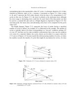
Before the twentieth century was very old, there were already several methods for repre-
senting endurance limit data. Under constant stress-controlled conditions, there are five
variables that can be used to characterize the fatigue cycle that is shown schematically in
Figure 2.10, only two of which are independent parameters:

max
, the maximum stress,

min
, the minimum stress,

mean
=
max
+
min
/2, the average or mean stress,

alt
=
max
−
min

/2, the alternating stress or half of the stress range, and
R =
min
/
max
, the stress ratio.
Characterizing Fatigue Limits 35
Stress
Time
Max
Mean
Min
R
= min/max
(a)
(b)
Figure 2.10. Schematic of (a) portion of a fatigue cycle included within (b) portion of a more complicated
combined LCF–HCF cycle.
The stress range is defined as the difference between 
max
and 
min
. An alternate nomen-
clature, used at times in industry, is the amplitude ratio defined as
A =

alt

mean
=

1−R
1+R
It is somewhat disappointing that, to this day, no general agreement has been reached
in the technical community regarding which pair of parameters should be used to char-
acterize a fatigue cycle. The reason for this is that each parameter has some physical
or mathematical significance, or is convenient to the user. For example, stress ratio, R,
may have no real physical significance, but many tests are conducted where R is the
parameter that is varied from one test to another and appears in the resultant database as
the constant under which the test was conducted. It was probably this type of thinking
and the number of available parameters that led the pioneers of HCF research to adopt
many different methods for representing endurance limit data. The diagrams on which
the data are represented can be classified as constant life diagrams, even though the intent
may have been for them to represent endurance limits. For practical purposes, tests were
often carried out to some reasonably long life, depending on the machines available, the
required number of tests or parameters to be varied, or the patience or available resources
of the investigator.
2.4. FATIGUE LIMIT STRESSES
The terminology “fatigue limit stress” or “strength” refers to the stress at a constant
(long) life that is normally used in place of the endurance limit (infinite life) in a constant
life diagram. Methods, particularly accelerated methods, for obtaining such stress values
are commonly obtained from S–N plots either by having data at the desired life or