High Cycle Fatigue: A Mechanics of Materials Perspective part 6 pdf

36 Introduction and Background
extrapolating data to the required life, often 10
7
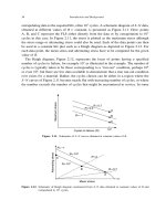
cycles. A schematic diagram of S–N data,
obtained at different values of R = constant, is presented as Figure 2.11. Here, points
A, B, and C represent the FLS either directly from the data or by extrapolation to 10
7
cycles in this case. In Figure 2.11, the stress is plotted as the maximum stress although
the stress range or alternating stress could also be used. Each of the data points can then
be used in a constant life plot such as a Haigh diagram as depicted in Figure 2.12. For
each data point, the mean stress and alternating stress have to be computed for the given
value of R.
The Haigh diagram, Figure 2.12, represents the locus of points having a specified
number of cycles to failure, for example 10
7
as illustrated in the example. The number of
cycles is typically taken to be those corresponding to a “run-out” condition, perhaps 10
8
or even 10
9
, but there are few data available to demonstrate that a true run-out condition
ever exists for a material. Rather, the cycles chosen can be either in a region where the
S–N curves of Figure 2.11 become nearly flat with increasing number of cycles, or where
the number exceeds the number of cycles that might be encountered in service. In some
Maximum stress
Cycles to failure (N )
R = 0.0
R
= 0.7
R = –1
10

7
A
B
C
Figure 2.11. Schematic of S–N curves obtained at constant values of R.
Alternating stress
R = 0
R
= 0.7
R
= –1
A
B
C
N
= 10
7
N = 10
4
Mean stress
Figure 2.12. Schematic of Haigh diagram constructed from S–N data obtained at constant values of R and
extrapolated to 10
7
cycles.
Characterizing Fatigue Limits 37
cases, neither condition may be satisfied. The points A, B, and C from Figure 2.11 are
shown in the Haigh diagram, Figure 2.12, corresponding to stress ratios, R, of 0.7, 0.0,
and −1, respectively. In this plot, alternating stress (half of the stress range) is plotted
against mean stress. Lines corresponding to these stress ratios are also shown, with the
vertical axis being the R =−1 line for fully reversed cycling. Although the Haigh diagram

is often presented or used with a straight line to represent data over a wide range of mean
stresses, there is no physical mechanism which requires the diagram to be linear over any
region. The straight line is often associated with the terminology “Goodman diagram,”
as discussed later in this chapter. The diagram is a locus of points obtained from a series
of experiments conducted under a range of values of R, and cases exist where it is highly
nonlinear. The Haigh diagram,
∗
a constant life diagram, could also represent the locus of
points at a lower life as depicted in Figure 2.12 for an arbitrary life of 10
4
cycles. This
usage, however, is not very common for establishing LCF limits.
The term “mean stress” is used in a Haigh diagram, although “average stress” or
“steady stress” is also commonly used. The steady stress is the stress level upon which
the vibratory stresses are superimposed, but the Haigh diagram represents only constant
amplitude loading, and does not represent a condition where variable amplitude or LCF
loading is superimposed. Further, the conventional Haigh diagram is valid only for the
frequency at which the data were obtained, which is typically less than that for which it
is applied in design. It is also not valid to use the Haigh diagram for random vibratory
loading without the existence of a validated cumulative damage model for HCF.
Although the majority of S–N data and curves are obtained under conditions at constant
values of R, some experiments, particularly on rotating components, are conducted under
conditions of constant mean stress. The difference between constant R and constant mean
stress is illustrated schematically in Figure 2.13. Recall that R is the ratio of minimum
to maximum stress. For constant mean stress cycles, each one will have a different value
of R. Conversely, cycles at constant R will have different mean stresses for different
values of stress range or maximum stress. Consider a material whose S–N behavior is
described by an equation of the form
logN =
0

+
1
logS −
2
 (2.1)
where 
0
and 
1
are fitting parameters, assumed for illustrative purposes, to be indepen-
dent of R. Note that this is a deterministic model and 
2
represents the endurance limit.
∗
The constant life or fatigue limit diagram that we refer to as the Haigh diagram, often incorrectly called the
Goodman diagram, has been referred to in early literature as an R–M diagram [15] or, alternately, as a R/M
diagram [16]. There, R refers to the range of stress (twice the alternating stress) while M refers to the mean
stress. The obvious confusion with stress ratio, R, probably led to other nomenclatures such as the (incorrect)
Goodman diagram, Haigh diagram, or alternating versus mean stress diagram.
38 Introduction and Background
Time
Stress
Constant R
Constant
mean stress
Figure 2.13. Schematic illustrating constant R and constant mean stress cycles.
To be consistent with fatigue thresholds typically being linearly decreasing functions of
R, we arbitrarily choose the following relationship to represent the endurance limit:

2

=150−100R (2.2)
In this numerical simulation, S is taken as the stress amplitude in arbitrary units. Using
constants 
0
=10 and 
1
=−2S–N curves are constructed as shown in Figure 2.14.
If the same equation is used to construct S–N curves at constant values of mean stress,
the resulting curves are as shown in Figure 2.15. The numerical values were taken only
for values of R between 0 and 1. Thus the range of mean stresses where a complete S–N
curve over the range of log N between 5 and 10 for this numerical exercise, is somewhat
limited. For this particular illustration, the constant mean stress curves have the same
general shape as the constant R curves but seem to be bunched together more. However,
this aspect of presenting the curves is highly dependent on the shape of the S–N curves
for the particular material.
0
100
200
300
400
500
5678910
R = 0
R = 0.5
R = 0.8
Stress amplitude
Log N
Figure 2.14. S–N curves for a hypothetical material at constant R.
Characterizing Fatigue Limits 39
0

100
200
300
400
500
5678910
σ
mean
= 150
σ
mean
= 300
σ
mean
= 500
Stress amplitude
Log N
Figure 2.15. S–N curves at constant values of mean stress.
An example of data obtained at several values of mean stress is presented in Figure 2.16
for a SKH51 tool steel [17]. While extrapolation and interpolation of data sets are
often necessary, the data in Figure 2.16 illustrate that single parameters with which to
consolidate data sets are not always viable because the individual groupings of data, at
constant mean stress in this case, do not follow well-behaved trends. In this case, the
slopes on the S–N curves do not change continuously with increase or decrease in mean
stress. Further, the cycles to failure where the curves become horizontal, indicating a
fatigue limit, also do not follow a consistent trend. Converting this data set to one where
stress ratios, R, are constant, is not very practical if formulae exist for interpolating or
extrapolating constant R data. This subject is discussed further in Chapter 8.
0
500

1000
1500
2000
10
3
10
4
10
5
10
6
10
7
10
8
Failure
Run-out
Stress amplitude (MPa)
Cycles to failure
σ
m
= –784 MPa
σ
m
= +784 MPa
σ
m
= 0 MPa
Figure 2.16. S–N data on SKH51 tool steel obtained at constant mean stresses [17].
40 Introduction and Background

While most of the data in many cases are obtained at R =−1, representing fully
reversed loading with no mean stress, the application of the Haigh diagram to HCF often
involves conditions at high values of R such as 0.7–0.9. These conditions represent high
mean stresses with small, superimposed vibratory stresses. There are often very few data
available in this region, and the extrapolation of data from low values of R and the
assumption that statistical distributions of data are the same at high R as they are at low
R are questionable.
Material quality is another parameter which has to be considered when using the Haigh
diagram in the design process. If the data are obtained in the laboratory on smooth
specimens, heat treatment, processing, microstructure, surface finish, and specimen size
must all be considered when applying the data to structural components. Perhaps, the
single most critical issue in the use of a Haigh diagram is the degree of initial or
service-induced damage which the material in the component may contain when such
damage is not present in the material used for the database. If, for example, microcracks
or other damage develops in service, then the High diagram has no meaning for this
material because it represents “good” or undamaged material. A design methodology
which considers the development of damage from any other source than the constant
amplitude HCF loading must be used to account for the different state of the material.
For example, if cracks develop due to LCF, then the tolerance of the material might be
evaluated using fracture mechanics and the concept of threshold stress intensity factor.
The Haigh diagram has no validity under this situation. It is these type of issues that are
addressed in the remainder of this book.
One method of developing a Haigh diagram which represents material in a component
is to develop the data on actual hardware. In this case, a combination of LCF and HCF
loading, or general spectrum loading, could be used to obtain a single point on the
diagram. Connecting this point to any other point on a Haigh plot has no physical basis
and no meaning, and most probably will be misleading. Unless the data are obtained under
purely HCF loading, with no other contributing damage mechanisms, the Haigh diagram
has no basis for use in design and the data would be better used in tabular fashion for
specific design conditions. It is relevant to note that trying to mix LCF and HCF data on

a single diagram is dangerous because the physical processes are different. LCF usually
involves high amplitude, low frequency loading, which leads to crack initiation early
in life and a considerable fraction of life under crack propagation. It is this aspect that
has allowed for the successful application of damage tolerance using fracture mechanics
in design. HCF, on the other hand, generally involves low amplitude, high frequency
loading, with a considerable portion of life spent in crack initiation. Interaction of the two
types of loading, therefore, can involve a process of crack initiation and growth under
LCF, and subsequent propagation under HCF. The Haigh diagram only represents the
HCF initiation portion in the absence of initial cracks and, therefore, has no meaning
under combined LCF–HCF loading. This topic is discussed in detail later in Chapter 4.
Characterizing Fatigue Limits 41
2.5. EQUATIONS FOR CONSTANT LIFE DIAGRAMS
To illustrate the different methods of representing data graphically, we consider several
models or equations that have been used traditionally for constant life diagrams [18].
The first and probably most popular is the Goodman line or equation, more commonly
referred to as the straight line in the modified Goodman diagram. It was actually proposed
by Haigh [19] in 1917 as a method for representing constant life, so the diagram that
plots alternating stress as a function of mean stress is not really a Goodman diagram
but a Haigh diagram and is thus referred to as such throughout this book. While some
of the equations to be discussed later are used to represent FLS data in Haigh diagram
plots, many have generally been established from empirical fits to data and have no
scientific basis. However, some of the earliest works tried to establish physical principals
for fatigue [18]. Goodman [20] proposed use of the “dynamic theory,” which is explained
in detail by Fidler [21], where it is assumed that vibratory loads produce the same
effect on a material as a suddenly applied load. Thus, vibratory loads are considered to
instantaneously produce stresses that are double those as if they were applied slowly. The
consequence of this is that the sum of the mean load and twice the alternating load should
not exceed the static ultimate strength of a material in order to have infinite fatigue life.
This results in a straight line on a Haigh diagram when the allowable alternating stress
is taken equal to half the ultimate stress (see Figure 2.17). Of interest is that Goodman

proposed such an equation as one that is “very easy of application and is, moreover,
simple to remember” [20]. He also noted that “whether the assumptions of the theory are
justifiable or not is quite an open question.” While the dynamic theory was simple, it was
observed that experimental data on all materials did not agree with the theory. To better
0
0.25
0.5
0.75
1
0 0.25 0.5 0.75 1
Stress/ultimate stress
Mean stress/ultimate stress
R

=

0
Ultimate stress
σ
vib
=

σ
ult
σ
vib
=

σ
ult

/2
Goodman line
Figure 2.17. Schematic of Goodman diagram showing allowable vibratory stress.
42 Introduction and Background
address true material behavior, the fully reversed alternating stress was adopted as an
empirical constant rather than half of the ultimate strength. What was originally termed
the “modified Goodman diagram” involved using straight line fit on a Haigh diagram
based on the experimentally determined fully reversed loading data point(s). The so-called
Goodman equation (or Modified Goodman equation) represented in the following plots
is of the form

a
=
−1

1−

m

u

(2.3)
where subscripts a, m, and u refer to the alternating, mean, and ultimate stresses, respec-
tively, and 
−1
represents the experimental value of the alternating stress under fully
reversed cyclic loading (R =−1). An alternate form of the Goodman equation is a straight
line that intersects the mean stress axis at the yield stress, 
y
, as opposed to the ultimate

stress. Such a representation of a fatigue limit constant life diagram was suggested by
Soderberg [22] and the equation is named after him in the literature.

a
=
−1

1−

m

y

(2.4)
To possibly better represent experimental data, a parabolic equation attributed to Gerber
[23] has been used which is of the form

a
=
−1

1−


m

u

2


(2.5)
Summarizing available fatigue limit data on a Haigh diagram, Forrest [15] observed
from a large body of data on ductile metals that 90% lie above the Goodman line and two-
thirds between the Goodman line and the Gerber parabola. He concluded that “although
not 100% safe, the Goodman line can therefore be recommended as a useful working
rule in design, when the fluctuating stress fatigue data are not available.” He cautioned,
however, that these conclusions do not necessarily apply to parts containing stress raisers.
There are a number of other representations of constant life data points [18], but one
more that achieved some popularity in the 1870s is known as the Launhardt–Weyrauch
(L–W) formula, developed by Launhardt [24] for positive values of R and extended by
Weyrauch [25] for negative values of R. Using 
u
as the ultimate stress, the equations are

max
=
0
+
u
−
0
R R > 0 (2.6)

max
=
0
+
0
−
−1

R R < 0 (2.7)
where subscript max refers to the maximum stress and 
0
and 
−1
refer to the maximum
stress at R =0 and R =−1, respectively. For the three formulas, the Modified Goodman
Characterizing Fatigue Limits 43
equation, the Gerber equation, and the L–W formulas, experimental data of Wöhler on
Krupp steel were used to establish a best-fit curve.
The first method of representing data is the diagram where maximum stress is plotted
against minimum stress, as shown in Figure 2.18. It can be seen that the Launhardt–
Weyrauch (L–W) formula and the Gerber parabola are almost identical in their repre-
sentation of the data (not shown). The straight line attributed to Goodman does a lesser
job of fitting data. The line representing minimum stress was often drawn to indicate
the lower stress boundary for admissible stress. The distance between the minimum and
maximum curves is then the allowable vibratory stress. In this and subsequent plots, the
curves are shown in terms of normalized stresses with respect to the ultimate stress. It
was Goodman [20] who stated that fatigue behavior should depend on the ultimate stress,
not the elastic limit.
Another way of representing constant life data is a plot of maximum and minimum
stress against stress ratio, as shown in Figure 2.19. Note that the Gerber and L–W
equations look almost identical again while the Goodman line is somewhat different. In
this particular plot, the linearity of the Goodman line disappears because of the particular
axes being used. This may be one reason why this type of plot has never retained any
popularity in the fatigue community.
A third type of plot, where maximum and minimum stresses are plotted against mean
stress, is shown in Figure 2.20. This plot probably contains the most information of use
to a designer of rotating machinery because mean stresses are not only well determined
from calculations based on centrifugal loads, but can also be well controlled in usage.

Alternating stresses that result from the vibration characteristics of the machinery are
much less controllable and not as well known in most cases. At high mean stresses (high
0
0.2
0.4
0.6
0.8
1
–0.5 –0.25 0 0.25 0.5 0.75 1
Goodman
Gerber
L–W
Maximum stress/UTS
Minimum stress/UTS
Minimum
Figure 2.18. Maximum and minimum stress as a function of minimum stress.
44 Introduction and Background
–0.5
0
0.5
1
–1 –0.5 0 0.5 1
σ
max
Goodman
σ
min
Goodman
σ
max

Gerber
σ
min
Gerber
σ
max
L–W
σ
min
L–W
Stress/UTS
Stress ratio, R
Figure 2.19. Maximum and minimum stress as a function of stress ratio, R.
–0.5
0
0.5
1
0 0.2 0.4 0.6 0.8 1
σ
max
Goodman
σ
min
Goodman
σ
max
Gerber
σ
min
Gerber

σ
max
L–W
σ
min
L–W
Stress/UTS
Mean stress/UTS
Figure 2.20. Maximum and minimum stress as a function of mean stress.
values of R), the maximum stress can become the governing stress for design because it
can approach the yield or ultimate strength of the material. The difference between the
two curves is the stress range, or twice the alternating stress. In this as in the previous
plots, the Gerber and L–W equations look nearly identical while the Goodman line, which
is now straight, differs a little from the other two equations.
The final method of plotting data is a plot of alternating stress against mean stress,
commonly but incorrectly referred to as the Goodman diagram, Figure 2.21. What should
Characterizing Fatigue Limits 45
0
0.1
0.2
0.3
0.4
0.5
0 0.2 0.4 0.6 0.8 1
Goodman
Gerber
L–W
Alternating stress/UTS
Mean stress/UTS
Figure 2.21. Alternating stress as a function of mean stress.

be properly called a Haigh diagram has evolved into the most commonly used method of
plotting FLS or endurance limit stress data, but the use of a straight line fit to the data
still seems to be popular.
The diagram most closely related to these methods of representing fatigue limit or
constant life data is the actual Goodman diagram shown in Figure 2.22, taken directly
from Goodman’s book [20]. The two curves shown in the figure are labeled maximum
and minimum stress. They are apparently plotted against minimum stress, as shown in
Figure 2.18, although there is no label on that plot or on the y axis. Regions of tension
and compression are shown above and below a zero stress line. Of greatest significance
in this plot, closest to what may be called a true Goodman diagram, is that the lines used
to represent the fatigue limit are straight lines on this particular plot. This is consistent
with the straight line formulation of Goodman shown in Figure 2.18 by comparison.
The L–W equations, shown in previous plots, can also be examined on a Haigh diagram.
For positive values of R, Equation (2.6) the shape of the curve depends on the value of

0
, the maximum stress at R =0. In a non-dimensional plot, where stresses are divided by

u
, the curves obtained for several values of 
0
/
u
are plotted in Figure 2.23. The label
“
0
” refers to the normalized value of 
max
at R =0. When 
0

= 1, the Haigh diagram
represents the points where 
max
=
u
for all values of R and is a straight line as shown.
For other values of 
0
, the lines are curved. Only the equation for positive values of R is
plotted in the figure. The line representing R =0 is shown, so the curves are valid only
to the right of that line. It is now obvious why the equation, valid now for positive R,
was modified to fit data at −1 <R<0 as given in Equation (2.7). For this range of R,
the points representing R =0 and R =−1 are connected by a smooth curve with slight
curvature (not shown here). The curve in Figure 2.23 for 
0
=05 goes through the point