High Cycle Fatigue: A Mechanics of Materials Perspective part 7 ppsx

46 Introduction and Background
1.0
0.8
0.6
0.4
0.2
–0.2
–0.4
–0.4 –0.2 0 0.2 0.4 0.6 0.8 1
Static breaking stress
Maximum stress
Minimum stress
Zero stress
Compression
Tension
Figure 2.22. Goodman diagram as shown in Goodman, 1899 [20] on p. 455.
0
0.2
0.4
0.6
0.8
1
0 0.2 0.4 0.6 0.8 1
σ
0
= 1
σ
0
= 0.75
σ
0

= 0.5
σ
0
= 0.25
Alternating stress/ultimate stress
Mean stress/ultimate stress
R = 0
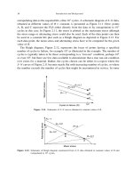
Figure 2.23. L–W equation for R>0 plotted on a Haigh diagram.
Characterizing Fatigue Limits 47
from the original Goodman equation at R =0 where 
max
=05
u
. The curve is closer to
a Gerber parabola than a straight line in that region but may not have any more physical
significance than the other two representations of experimental data.
It can be seen that the development of methods to represent fatigue limit data was based
on a combination of mathematically simple forms as well as graphical representations.
While there seemed to be a physical basis of some sort for all of the approaches, combined
with simplicity, it should be pointed out that the choices of methods of representing
data were scrutinized throughout their development. A particularly insightful example of
such a critique was made in 1880 [26], although similar words would be equally valid
today. Commenting on the W–L formula, used to fit Wöhler’s data, Smith writes, “In
fact, the formula seems to be more the product of pure imagination than to be based
on the experiments.” He further points out that “the formula can, of course, be made to
agree with the extreme results of any particular set of experiments. What I, and I dare
say some others, would like to know, is whether this formula agrees with even a rough
degree of approximation with the intermediate results.” He goes on to question “whether
the parabolic curve . is the correct curve ” and sums up: “I submit that the proper
thing to do is not to coin rules out of imagination, but to persevere in careful and patient

experiments, and to watch narrowly and to study and analyze closely the results until the
true intimate laws of the stress and fatigue of metals are revealed.”
2.6. HAIGH DIAGRAM AT ELEVATED TEMPERATURE
In the final program on HCF material behavior [27], a Haigh diagram was constructed
for a single crystal alloy, PWA 1484 at a life of 10
7
cycles based on 1900

F S–N test
data. The stress-life behavior was characterized for each stress ratio, R, in terms of the
alternating stress 
alt
using a power law relationship:
N
f
=k
m
alt
(2.8)
Data were used only from <001> oriented specimens with the exception of eight spec-
imens oriented at < 001+15> that were tested at R = 08. The <001 +15> oriented
data fall on top of the < 001> data and consequently were included in the data set to
characterize the R = 08 stress-life behavior. Values for the constants k and m for each
tested value of R are shown in Table 2.1.
Using the empirical S–N relationships, the curve was extrapolated to longer lives and
a Haigh Diagram was constructed corresponding to a life of 10
7
cycles, as shown in
Figure 2.24.
The Haigh diagram shows the HCF capability of PWA 1484 at 1900


F. The shape
of the diagram is fairly conventional for low values of mean stress. A gradual decrease
48 Introduction and Background
Table 2.1. Constants for S–N empirical fits at 1900

F
Rmk
−1 −12420E +27
−0333 −3019E+11
01 −5956E+14
05 −4910E+12
08 −7519E+11
0
10
20
30
40
50
01020304050
59 Hz HCF data
Alternating stress (ksi)
Mean stress (ksi)
R = –1
R
= –0.33
R
= 0.8
R
= 0.5

R
= 0.1
46 Hr Rupture capability
Figure 2.24. 1900

F Haigh diagram for PWA 1484, 10
7
cycles.
in alternating stress capability is accompanied by an increase in allowable mean stress.
However, above R =05, the alternating stress capability drops off rapidly as the stress
rupture capability is approached. The stress rupture capability can be represented as an
asymptote at R = 1 at 46 hours, the time for 10
7
cycles at 60 Hz (which was the original
planned frequency). For this material, there are both cycle-dependent and time-dependent
modes of failure, the former normally associated with the value of the alternating stress
and the latter associated primarily with the mean stress.
To account for this more complex fatigue behavior, a Walker model was used to
represent the behavior of the material. In the Walker model, an equivalent alternating
stress is defined to take into account different mean stress conditions. This equivalent
alternating stress, 
equivalent_alt
, is then used in the stress-life power law relationship as
shown below:
N
f
=k
equivalent_alt
m
(2.9)

where the equivalent alternating stress is given by:

equivalent_alt
=
alt
1−R
W −1
(2.10)
Characterizing Fatigue Limits 49
The Walker exponent, w, was determined by taking data from several values of R
and iterating until the standard error in predicted life was minimized. The Walker model
collapsed the S–N response over a range of stress ratios. While the Walker exponent is
normally determined over the full range of stress ratio data that are available, in this case
R =−1toR = 08, the goal here was to capture only those specimens failing in a pure
fatigue mode. Fractography showed that failure was dominated by fatigue only at low
stress ratios or low mean stress loading conditions.
Two approaches were considered for fitting the Walker model. The first (termed
“Walker model A” in what follows) used 59 Hz HCF data at all R ≤ 01. A second
approach (Walker model C) was examined because despite the fatigue-based appearance
of specimens at R = 01 tested at 59 Hz, previous work showed that a time-dependent
process is also present at this test condition [27]. At a constant stress level at R =01,
fatigue life in cycles increased as the frequency was increased from 59 to 900 Hz.
A linear line with a slope of 1:1 approximated the data fairly well indicating a fully
time-dependent process up to the highest frequency that was tested, 900 Hz. A transition
to time-independent behavior with cycles to failure maintaining a constant level may exist
just beyond 900 Hz or could occur well beyond that frequency. As a result, the estimate
of the Walker exponent for pure HCF may be affected by using the lower 59 Hz data.
Therefore the second approach used only high frequency data (370–400 Hz) at R =01in
combination with 59 Hz data at R =−1 and R =−0333 to represent time-independent
behavior. Walker model constants for each subset of HCF data are shown in Table 2.2.

In Figure 2.25, Walker model A approximates the 59 Hz HCF data fairly well up to
a value of R = 01. Walker model C shows a benefit in alternating stress capability at
R =−0333 and R = 01 compared to the other models. Both Walker models deviate
from the 59 Hz Haigh diagram above R = 01 since the mean stress increases and time-
dependent failure mechanisms reduce the cyclic capability of the material.
To account for the time-dependent behavior of the material, two approaches were used
in modeling the rupture behavior of PWA 1484 at 1900

F. The first approach, the simpler
of the two, assumes that only the applied mean stress contributes to rupture damage.
This approach is referred to as the Mean Stress Rupture Model. The second method,
the Cumulative Rupture Model considers the summation of rupture damage from applied
stress over the entire fatigue cycle.
Table 2.2. Constants for 1900

F Walker models
Walker model HCF Data subset Number of tests k m Walker exponent, w
A R ≤−01 @ 59 Hz 24 5.83E16 −717 0165
C R ≤−0333 @
59HzR= 01
@ 370–400 Hz
20 7.63E16 −698 03817
50 Introduction and Background
0
10
20
30
40
50
01020304050

59 Hz HCF data
Walker model A
Walker model C
Alternating stress (ksi)
Mean stress (ksi)
Figure 2.25. Walker models A and C with 59 Hz 10
7
cycles Haigh diagram.
The Mean Stress Rupture Model is represented by the expression in Equation (2.11)
that relates mean stress to time to rupture. The expression was derived by fitting a power
law relationship to four tests that were conducted until rupture. The resulting equation is
t
f
=219×10
9

−5069
mean
(2.11)
where 
mean
is the applied mean stress in ksi and t
f
is the time to failure in hours.
In the Cumulative Rupture Model, the rupture damage due to the applied stress is
integrated over the cyclic load and the applied stress is expressed as a sinusoidal function
using  as the period of the cycle in hours. To do this, the load cycle is divided into
small time increments, t. At each time increment, the applied stress is calculated and
the corresponding rupture life is determined using Equation (2.10). The rupture damage
for the time increment is calculated and damage fractions for t are summed over the

loading cycle. The number of cycles to failure can be calculated using the assumption
that failure occurs when the rupture damage equals one.
When R is less than zero, a portion of the loading cycle is compressive. Two scenarios
were considered when applying the Cumulative Rupture Model: (a) compressive stress
is neither damaging nor beneficial to life, and (b) compressive stress is damaging to life.
Thus, in total, three rupture models were considered: Mean Stress Rupture Model, Cumu-
lative Rupture without compressive damage, and Cumulative Rupture with compressive
damage.
Figure 2.26 shows the rupture model predictions for a constant life of 10
7
cycles at
59 Hz compared to the HCF test data. Both cumulative rupture models approximate the
shape of the Haigh diagram based on the experimental data. The mean stress model
predicts a mean stress of 32.5 ksi independent of R for 10
7
cycles at 59 Hz since the model
is purely time-dependent and does not consider any cyclic contribution to the damage
process. It is worth noting that the cyclic models, Figure 2.25, seem to do a good job
Characterizing Fatigue Limits 51
0
10
20
30
40
50
0 1020304050
59 Hz HCF data
Cumulative rupture, no compressive
damage
Cumulative rupture with compressive

damage
Mean stress rupture model
Alternating stress (ksi)
Mean stress (ksi)
R = –1
R
= –0.33
R
= 0.8
R
= 0.5
R
= 0.1
Figure 2.26. 1900

F10
7
cycle Haigh diagram at 59 Hz with rupture model predictions.
of fitting the data at low values of mean stress. They are derived, however, from fitting
those very same data. The rupture model predictions, on the other hand, are derived
strictly from rupture data with no cyclic content. The ability of the rupture models to
represent data over the entire range of mean stresses, Figure 2.26, seems to indicate that
the behavior of PWA 1484 at 1900

F is purely time-dependent, or, at least for modeling
purposes, can be treated as such.
The example cited above points out some of the considerations that are encountered
when plotting data on a Haigh diagram and then trying to interpret the data or model
the material fatigue limit when the material behavior includes time dependence. Factors
such as cyclic frequency become important considerations and, at a minimum, should be

indicated in Haigh diagram plots.
2.7. ROLE OF MEAN STRESS IN CONSTANT LIFE DIAGRAMS
In dealing with data on FLSs, it is common to plot these stresses as a function of stress
ratio (R = ratio of minimum to maximum stress), or, more commonly, of mean stress. The
Haigh diagram, incorrectly referred to as a Goodman diagram, is a common method of
representing the fatigue limit or endurance limit stress of a material in terms of alternating
stress, defined as half of the vibratory stress amplitude. Thus, the maximum dynamic
stress is the sum of the mean and alternating stresses. For many rotating components,
the mean stress is known fairly accurately, but the alternating stress is less well defined
because it depends on the vibratory characteristics of the component. Thus a Haigh
diagram represents the allowable vibratory stress as the vertical axis as a function of
mean or steady stress as the x axis. While attempts have been made to define the equation
which best represents the data on a Haigh diagram, as described earlier in this chapter,
52 Introduction and Background
variability from material to material, scatter in the data, and lack of sufficient data in
many cases prevent the fitting of an equation to such data.
When mean stress values are negative, or for values of R less than minus one, there are
very few data and no general guidelines for extrapolating equations which were meant
to represent data on a Haigh diagram only for positive values of mean stress. In cases
such as contact fatigue, very high compressive stresses can be present, necessitating
knowledge of fatigue behavior or fatigue limits for negative mean stresses. One of the
most important areas where negative mean stresses can occur is in the case of the
introduction of compressive residual stresses into a material or component. Shot peening,
for example, is commonly used as a surface treatment to improve the fatigue properties
of a material by introducing residual compressive stresses into the material up to depths
typically no greater than 0.1 mm. While compressive stresses in the vicinity of the surface
reduce the maximum stress from vibratory loading at the surface, they do not reduce
the vibratory amplitude. Thus, in effect, they drive the mean stress lower, often into the
compressive regime. While these residual compressive stresses are known to improve
the fatigue characteristics in many materials and geometries, they are generally not taken

into account in design and are used, instead, to improve the margin of safety. If such
a condition is to be taken into account in design, a thorough understanding of material
behavior and fatigue limits under negative mean stresses is required. The subject of
residual stresses and accounting for them in design is discussed in Chapter 8.
Forrest [15] has assembled a large body of fatigue limit strength data on ductile metals
and plotted them in dimensionless form as indicated in Figure 2.27. The thick straight
Mean stress /yield stress
–1
Alternating stress/s
–1
2.0
1.5
1.0
0.5
–1.0 –0.5 0 0.5 1.0
Figure 2.27. Schematic of observed behavior at negative mean stress.
Characterizing Fatigue Limits 53
line represents the data (not shown) quite well and illustrates that extending the fit
into the mean stress regime produces alternating stress values that continue to increase
with decreasing mean stress. The data chosen by Forrest [15] for this type of plot were
filtered from available data to meet a criterion to accept only those results where special
precautions were taken to insure axiality of loading. The data covered a range of aluminum
and steel alloys. As noted earlier, when discussing the effects of compressive residual
stress on fatigue limit strength, Forrest [15], in 1962, already recognized the importance
of the shape of the curve fit to the data by stating that the “behaviour is particularly
significant with regard to the effect of residual stresses on fatigue strength.”
Representing compressive mean stress data on Haigh or other types of diagrams
described above was never much of a consideration because data obtained at mean stresses
below zero, corresponding to fully reversed loading or R =−1, essentially did not exist.
We now examine the capability of equations to represent negative mean stress data.

In addition to the modified Goodman equation and the others described above, there
have been many variations of straight lines and other curves to try to represent fatigue
limit data for HCF design. Additionally, there are fatigue equations that are used mainly
to fit data in the LCF regime, which try to account for the effects of mean stress or stress
ratio by introducing a single parameter to consolidate such data. Two such equations are
the one due to Smith, Watson, and Topper (SWT) [28] and the commonly used Walker
equation. For the SWT equation, an effective stress is given in terms of maximum stress
and strain range. In HCF, elastic behavior is assumed, thus strain range and stress range
can be used interchangeably when dealing with FLS conditions. The SWT equation for
elastic behavior is in the form

eff
=
−1
=


max

2

1/2
=
max

a

1/2
(2.12)
where 

eff
can be treated as a constant,  is the stress range,  =2
a
, and 
max
is the
maximum stress. The fully reversed R =−1 stress, both the maximum and alternating
value, is denoted by 
−1
. This equation is plotted in the form of a Haigh diagram in
Figure 2.28 using a value of 
eff
=200 MPa which is representative of data on a forged
titanium bar material [29]. The exponent in Equation (2.12) is taken as the one used
most commonly, namely 0.5. For reference purposes, the Jasper equation, discussed later,
is plotted because it is found to describe the shape of the Haigh diagram for positive
mean stress quite well. Of greatest interest in Figure 2.28 is the shape of the curve for
the SWT equation for negative mean stress, which shows an ever increasing alternating
stress as mean stress becomes further negative. As an alternative, if we choose to take
half the strain range (or half the stress range) as that corresponding to positive stresses
only ( =+in the figure), this changes the curve only slightly in the negative mean
stress regime. Note, finally, the symmetric shape of the Jasper equation about zero mean
stress. This also will be discussed later.
54 Introduction and Background
0
200
400
600
800
1000

–400 –200 0 200 400 600 800 1000
SWT
² σ = +
Jasper
Alternating stress (MPa)
Mean stress (MPa)
Figure 2.28. Haigh diagram representation of SWT and Jasper equations.
A similar treatment can be given to the Walker equation which, as for the SWT
equation, is commonly used to consolidate LCF data obtained at different stress ratios, R.
The equation is similar to the SWT equation, but adds a degree of flexibility through the
exponent w. It has the form

eq
=2
w

−1
=
w

max

1−w
(2.13)
where w is the Walker exponent. With the exception of the value of the coefficient in
Equation (2.13), it is identical in form to the SWT equation when w =05. Figure 2.29 is
a plot of the Walker equation for various values of the exponent w, including extension
of the equation to account for negative mean stress or values of R<−1. The curves are
all forced to go through the same point at zero mean stress. While some data are handled
by changing the value of w for negative values of R, it can be seen that the Walker

equation has the same general characteristics as the SWT equation for negative mean
stress, namely that alternating stress continues to increase as mean stress goes further
negative. Further, for both equations, the shape of the curves for positive mean stress is
concave up over the entire region.
Several attempts were made in the early days of fatigue modeling to account for the
observed behavior of the FLS when the mean stress was negative. In 1930, Haigh [30]
pointed out that experimental data indicate that the constant life diagram is not symmetric
Characterizing Fatigue Limits 55
0
200
400
600
800
1000
–400 –200 0 200 400 600 800 1000
w = 0.2
w = 0.3
w = 0.4
w = 0.5
w = 0.6
w = 0.7
Alternating stress (MPa)
Mean stress (MPa)
Constant life diagram
Walker equation
Figure 2.29. Haigh diagram representation of Walker equation.
with respect to 
m
as required by the Gerber and generalized Goodman formulas.
∗

He
suggested that the data can be represented by the generalized parabolic relation

a
=
−1

1−k
1


m

u

−k
2


m

u

2

(2.14)
where the constants k
1
and k
2

are selected to give the best fit of the data. A plot of
this equation is presented in Figure 2.30 for several combinations of k
1
and k
2
while
constraining the curves to go through the ultimate stress point on the x axis and the
alternating stress value at R =−1onthey axis. The case where k
1
=0k
2
=1 represents
the Gerber parabola, Equation (2.5), symmetric about the y axis. When k
1
=1 and k
2
=0,
the modified Goodman line is obtained, extrapolated for negative mean stress.
More complex equations have been proposed, such as that by Heywood [31], who used
an empirical cubic equation for representing constant life data. His equation has the form

a
=

1−


m

u



−1
+
u
−
−1


(2.15a)
∗
While the generalized Goodman equation [3] does not indicate symmetry with respect to 
m
, the formulation
in the first Edition of Goodman’s book [20] presents equations for the static load capability in terms of the
dynamic theory. If it is assumed that the strength is equal in tension and compression, the equations indicate
that there is symmetry with respect to mean stress. The lack of data for negative mean stresses prevented
any substantial debate on this issue of symmetry. The symmetry of the Goodman equation and its history are
discussed in [18].