High Cycle Fatigue: A Mechanics of Materials Perspective part 8 ppsx

56 Introduction and Background
0
0.5
1
1.5
2
–1 –0.5 0 0.5 1
Haigh equation
k
1
= 0.0, k
2
= 1.0
k
1
= 0.25, k
2
= 0.75
k
1
= 0.5, k
2
= 0.5
k
1
= 0.75, k
2
= 0.25
k
1
= 1.0, k

2
= 0.0
σ
mean
/σ
ult
σ
alt
/σ
ult
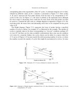
Figure 2.30. Constant life diagram for parabolic equation of Haigh.
 =


m

u

e +g


m

u

(2.15b)
where e and g are either positive or negative constants. Because of the large number of
terms, most experimentally determined constant life data may be represented by proper
selection of the constants.
2.8. JASPER EQUATION

Of both practical and historical significance is the observation that Jasper [32], in 1923,
proposed that fatigue life is related to the stored energy density range per cycle in
a material when evaluating data obtained earlier by Haigh. Applying this concept to
HCF conditions, it can be assumed that all stresses and strains are elastic, thus all
equations represent purely elastic behavior. For purely uniaxial loading, the shaded area
in Figure 2.31 illustrates schematically the stored energy for the cases where loading is
purely tensile R > 0. The energy for the case where R<0, which involves tension and
compression in a single cycle, is illustrated in Figure 2.32 by the shaded area. The stored
energy density range per cycle is then given for uniaxial loading by
U =


max

min
d=
1
E


max

min
d (2.16)
Characterizing Fatigue Limits 57
maxmin
σ
ε
Figure 2.31. Stored energy (shaded) for elastic loading under tension fatigue R > 0.
min

max
σ
ε
Figure 2.32. Stored energy (shaded) for elastic loading under reversed fatigue R < 0.
58 Introduction and Background
since  =EE is Young’s modulus. The energy can then be written as
U =
1
2E


2
max
±
2
min

(2.17)
where the plus sign is for R<0 and the minus sign for R>0 (see Figures 2.31 and
2.32). For purposes of presenting the equation in the form of a Haigh diagram, the stress
limits are written in terms of mean and alternating stresses

max
=
m
+
a
(2.18a)

min

=
m
−
a
(2.18b)
where 
m
and 
a
represent the mean and alternating stresses, respectively.
For the specific case of fully reversed loading, R =−1, the energy is written as
U =
1
2E
2
2
−1
 (2.19)
where 
−1
represents the alternating stress (= maximum stress) at R =−1. For any other
case of uniaxial loading, the following equation is easily derived and can be used to
obtain the value of the alternating stress on a Haigh diagram in terms of stress ratio, R:

a
=

−1
√
2


1−R
2
1−RR
(2.20)
where R is used to denote the absolute value of R. It follows that the alternating stress
when R = 0, defined as 
0
,is

0
=


−1
2
2
(2.21)
Of interest is the shape of the Haigh diagram corresponding to a constant energy density
range for any positive mean stress value. Such a diagram is shown in Figure 2.33 which
has the same general shape as that for Ti-6Al-4V bar material (Figure 2.34) obtained
by Maxwell and Nicholas [33]. It should be noted that only a single parameter, 
−1
,
is required to describe the values on both the x and y axes. This plot (Figure 2.33) is
the same type as shown previously as the Jasper equation in Figure 2.28, using typical
numbers for titanium plate, where the alternating stresses corresponding to negative mean
stresses are also included.
Data on another high strength titanium alloy, Ti-6-2-4-6, that extend into the negative
mean stress regime are shown in Figure 2.35. These data show the same general trend

as the Jasper equation curve of Figure 2.33 for positive mean stresses and have a shape
Characterizing Fatigue Limits 59
0
0.2
0.4
0.6
0.8
1
1.2
0 0.5 1 1.5 2 2.5 3 3.5 4
σ
alt
/σ
–1
σ
mean
/σ
–1
Normalized Haigh diagram
Jasper equation
Figure 2.33. Normalized Haigh diagram representing Jasper equation for positive mean stresses.
0
100
200
300
400
500
600
700
800

0 200 400 600 800 1000
Alternating stress (MPa)
Mean stress (MPa)
Ti-6Al-4V bar
10
7
cycles
70 Hz
Figure 2.34. Haigh diagram for Ti-6Al-4V bar [33].
similar to that shown subsequently in Figure 2.36 when extended into the negative mean
stress regime. The representation of data for negative mean stresses is discussed in the
following paragraphs.
Experimental data for negative mean stress were obtained by Nicholas and Maxwell
[29] that showed they neither followed the Jasper equation nor the SWT or Walker
equations (see Figure 2.28). For that reason, they proposed a modification to the Jasper
equation that treats the stored energy due to tension differently than that due to com-
pression stresses. Haigh [30], in 1929, in referring to Bauschinger’s results from 1915
60 Introduction and Background
0
100
200
300
400
500
600
700
800
–200 0 200 400 600 800 1000 1200
Ti-6-2-4-6
Alternating stress (MPa)

Mean stress (MPa)
10
7
cycles
60–70 Hz
Figure 2.35. Haigh diagram for Ti-6-2-4-6.
0
100
200
300
400
500
600
700
800
–400 –200 0 200 400 600 800 1000
ML data
ASE data
Jasper, α = 0.287
Alternating stress (MPa)
Mean stress (MPa)
Ti-6Al-4V plate
10
7
cycles
20–70 Hz
Figure 2.36. Haigh diagram for Ti-6Al-4V plate including modified Jasper equation fit.
and 1917, noted that “this series of tests  was probably the first that ever revealed
any difference between the actions of pull and push in relation to fatigue.”
∗

Referring to
data on naval brass, he indicated, “In this metal, as in many others, pull tends to reduce
the fatigue limit while push increases the resistance to fatigue.” Following this idea,
Nicholas and Maxwell postulated that stored energy density per cycle does not contribute
∗
“Push” and “pull” was the common nomenclature for tension and compression, respectively, in that time
period.
Characterizing Fatigue Limits 61
towards the fatigue process as much when the stresses are compressive as when they are
in tension. Taking the simplest approach, where compressive stress energy contributes
a fraction, , compared to comparable energy in tension, then the total effective energy
was formulated in the following manner, where <1:
U
tot
=U
tens
+U
comp
=constant (2.22)
In the use of this equation, energy terms corresponding to negative stresses have to
be modified by the coefficient . The introduction of the constant  has the effect of
modifying the shape of the Jasper equation as shown in Figure 2.37 for several values of
the constant . The stresses on both axes are the same as those used in Figure 2.28. The
constant  was then used to fit actual experimental data obtained at values of R<−1
corresponding to negative mean stresses.
Using the Ti-6Al-4V forged plate material, fatigue tests were conducted under constant
amplitude stress conditions over a wide range of stress ratios from 0.8 to −35. The mini-
mum stress ratio value at which tests could be conducted was limited by the compressive
yield strength of the material. To establish the fatigue limit strength corresponding to
10

7
cycles, samples were fatigue tested using the step-loading procedure of Maxwell and
Nicholas [33] that is discussed in the next chapter.
The experimental values for the FLS obtained for a broad range of values of R are
plotted in the form of a Haigh diagram in Figure 2.36. The data are shown as ML in the
figure, and are combined with previously unpublished data from Allied Signal Engines
(ASE), now Honeywell, on the same material. A best fit of the data using the modified
Jasper equation is also shown in the figure. The constant, , in the modified Jasper
equation (2.22) was obtained as 0.287 by fitting to the experimental data obtained from
0
100
200
300
400
500
600
–400 –200 0 200 400 600 800 1000
α = 1
α = 0.75
α = 0.5
α = 0.25
Alternating stress
Mean stress
Constant life diagram
modified Jasper
Figure 2.37. Haigh diagram for modified Jasper equation for various values of .
62 Introduction and Background
R =08toR =−35. The weighted energy was obtained for each data point as a function
of the variable  in Equation (2.22) and the percent least squares error between the
average energy of all the data points and the individual energy values was minimized.

To plot the resulting modified Jasper equation, the stress corresponding to the average
energy at R =−1 had to be obtained and was found to be 500MPa.
In reviewing the methods for representing fatigue limit data on constant life diagrams,
Maxwell and Nicholas [33] noted that the Haigh diagram is the one that has achieved
the most popularity. In a review of these diagrams, the authors suggested that the most
important information for design was not only the alternating stress, but also the maximum
stress, as represented in a plot against mean stress (see Figures 2.20 and 2.21 above).
To this end, a diagram called the Nicholas–Haigh diagram was proposed [33] which, as
history would note, received absolutely no acceptance or recognition from the technical
community and was short-lived, never to be mentioned again until here. For the sake
of posterity, the reasoning behind the proposed diagram, and more importantly, the
importance of maximum stress in constant life diagrams is discussed next.
The plot of both alternating stress and maximum stress against mean stress, initially
referred to as a Nicholas–Haigh diagram [33] is presented at the possible expense of
duplicating past efforts as well as confusing future historians. This plot can be used
to present data for engineering design in two fashions. For low values of mean stress
or low RR<05, the alternating stress is the crucial allowable quantity, particularly
for rotating machinery applications where mean stresses are relatively predictable and
normally are well defined. For high values of mean stress or high RR>05, maximum
stress becomes the more critical parameter in design. It is suggested here that margins of
safety be imposed on both parameters (alternating stress and maximum stress) in order
to insure a safe design. The Nicholas–Haigh diagram was an attempt to present data in a
form that would allow a designer to recognize the importance of both quantities. Such a
plot may not be totally new, but the following features were incorporated in it:
a. It is a method of representing experimental data. There is no equation or formula
intended or implied to represent the data.
b. There is no specific value of an y-axis intercept (zero mean stress or R =−1) which
is related to any material property such as yield or ultimate stress.
c. There is no value, experimental or theoretical, associated with an x-axis intercept
(R =0).

This last condition differs from most previous diagrams or laws that attempt to pin the
data to the ultimate strength for theoretical reasons, or to yield stress for engineering
purposes. One of the main reasons for avoiding an intercept such as the ultimate strength
is that ultimate strength depends on the strain rate at which a test is conducted, and
since most metals exhibit some degree of strain-rate hardening [34]. Data plotted on a
Characterizing Fatigue Limits 63
Nicholas-Haigh diagram are normally conducted at a single frequency which produces a
different strain rate for each different amplitude of alternating stress. For increasing values
of mean stress, as R approaches 1, the strain rate approaches zero since the alternating
stress amplitude is normally found to decrease in this region. This is equivalent to having
a cyclic stress–strain curve near the ultimate stress at an arbitrarily slow rate of loading.
Thus, a fourth condition can be suggested for a completely defined Nicholas–Haigh
diagram, namely, that the frequency of loading for all data points be specified on the
diagram.
It should be noted that data for Haigh or other constant life diagrams for large cycle
counts, generally in excess of 10
7
for HCF applications, are obtained at high frequencies.
Thus, the strain rates associated with such tests are not quasi static. For this reason,
maximum stress values obtained under fatigue testing at high values of R and high
frequency can often be above the quasi-static ultimate strength of the material. This, in
turn, will not produce a smooth plot on a Haigh diagram if a quasi-static ultimate strength
is used to anchor the plot to the x-axis.
As a further consideration, it is recommended that all data points be included, partic-
ularly those obtained at high values of RR→1. In this region, many materials tend
to exhibit creep behavior which may lead to a creep rather than a fatigue failure (see the
discussion in Chapter 3 on testing at high stress ratios as well as the earlier discussion
on Haigh diagrams at elevated temperature). Nonetheless, if the frequency is specified,
the time to failure can be easily deduced. Data of this type should be appended with a
footnote if necessary, but they are still valid design data, even though the mode of failure

is not pure fatigue.
In the limit, a “fatigue” test at very high values of R becomes a creep or sustained load
test. Any strain hardening which occurs due to strain rate effects, therefore, is influenced
by the rate of loading which is used in going from zero to mean stress during the first
half cycle at the start of the test. This rate of loading should be recorded, particularly if
data are to be compared with an ultimate stress value. The ultimate stress, consequently,
should be obtained from a test at the same rate of loading for consistency.
An example of a Nicholas–Haigh diagram is presented in Figure 2.38 for titanium alloy
Ti-6Al-4V. The data are those presented previously in Figure 2.36 and are represented
by the modified Jasper equation for both maximum and alternating stress. Note that the
maximum stress approaches and then exceeds the yield stress of the material (930 MPa)
at high values of mean stress.
It is of importance to note that the Haigh diagram, especially when extended into
the negative mean stress regime, provides useful information on the potential beneficial
effects of residual stresses. (Residual stresses and their role in endurance limits are
discussed in detail in Chapter 8.) Notwithstanding the fact that stress gradients play an
important role in fatigue, comparing allowable alternating stresses as a function of mean
stress can give guidance on the role that residual stress can play in altering the fatigue
64 Introduction and Background
0
200
400
600
800
1000
–400 –200 0 200 400 600 800 1000
ML data
ASE data
Jasper, α = 0.287
Jasper σ

max
Alternating stress (MPa)
Mean stress (MPa)
Ti-6Al-4V plate
10
7

cycles
20–70 Hz
Yield stress
Figure 2.38. Nicholas–Haigh diagram for Ti-6Al-4V plate with modified Jasper equation fit shown for alter-
nating stress (solid line) and maximum stress (dashed line).
limit strength. Noting again that compressive residual stresses do not alter the range of
stress or alternating stress applied to a material or structure but, rather, reduce the mean
stress, the Haigh diagram provides data on the reduction of the allowable alternating
stress as a function of mean stress. Using the Jasper equation as a measure of the
allowable alternating stress, if a material is subjected to a vibratory stress at R =0, with
an alternating stress magnitude denoted by 
0
, then the mean stress is also 
0
. Addition
of a compressive residual stress of an equal magnitude 
0
will then result in a mean stress
of zero which, in turn, will increase the allowable alternating stress by a factor of
√
2, as
seen from Equation (2.21). Yet if the original stress state is at R =−1, and a compressive
residual stress is added, then the modified Jasper diagram representing Ti-6Al-4V plate

material, Figure 2.36 shows that the benefit of compressive residual stress is somewhat
limited. In going from a mean stress of zero to a mean stress of −400MPa, for example,
Figure 2.36 indicates a benefit in allowable alternating stress of only approximately 20%
since the alternating stress of approximately 500 MPa only increases to approximately
600 MPa. This type of information can be easily seen in a plot of maximum stress against
mean stress, Figure 2.38, where the maximum stress corresponding to the fatigue limit
is seen to decrease as mean stress decreases in the negative mean stress regime. Thus, it
has to be ascertained where the mean stress is without residual stress and where the mean
stress will be after a compressive residual stress is developed. From that information,
the allowable alternating stress for the material can be determined and the benefit of the
residual stress ascertained. The subject of residual stresses and their effect on fatigue
behavior in conjunction with other considerations evolving from surface treatments is
discussed further in Chapter 8.
Characterizing Fatigue Limits 65
2.9. OBSERVATIONS ON STEP TESTS AT NEGATIVE R
Data obtained in [29] have been examined for implications on the initiation and subsequent
propagation of cracks in smooth bars cycled at negative stress ratios. The data, shown
above in a Haigh diagram in Figure 2.38, cover a range of stress ratios, R, from a high
value of 0.8 down to −35. They were fit to a modified form of the Jasper equation
which accounts for the different behavior in initiation in compression compared to that
in tension using the constant . In addition to the alternating stress normally provided in
a Haigh diagram, the maximum stress is also shown by a dashed line in the figure. The
data were obtained using the step-loading procedure, described in the next chapter, with
blocks of 10
7
cycles. Of significance is the number of cycles to failure in the last loading
block as a function of R shown in Figure 2.39. The relatively low number of cycles in
the last block leads to speculation that these specimens, at low values of R, had already
developed cracks in earlier cycle blocks and that these cracks did not propagate until
some higher stress level was reached in the final block. If, according to this speculation,

the crack propagates only due to positive stresses (positive K), then the cracks formed
at lower values of R must be larger than those at higher R because the maximum stress
(positive portion of cycle) decreases with decreasing R (see Figure 2.38). The indirect
evidence of small numbers of cycles in the last loading block is discussed further in
Chapter 3 when dealing with specimens that are deliberately precracked before endurance
limits are determined using step loading.
The speculation about crack initiation and subsequent propagation at negative R can
be explained with the aid of Figure 2.40, where the conditions for initiation compared
to propagation are shown schematically. The initiation of a crack, if associated with the
0 × 10
0
2 × 10
6
4 × 10
6
6 × 10
6
8 × 10
6
1 × 10
7
–4 –3 –2 –1 0 1
ML data
ASE data
Last block cycles
Stress ratio, R
Ti-6Al-4V plate
Smooth bar step tests
10
7

cycle blocks
60 Hz
Figure 2.39. Cycles to failure in last cycle block for smooth bar specimens.