High Cycle Fatigue: A Mechanics of Materials Perspective part 10 ppt

76 Introduction and Background
N
Mean stress
Alternating stress
R = constant R = constant
10
7
2 × 10
7
3 × 10
7
Alternating stress
σ
Goodman
σ
Goodman
Goodman diagram
Loading history
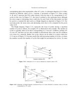
Figure 3.2. Schematic of step-loading procedure.
others do not because the test is terminated after a large number of cycles (run-out). This
results in two populations of specimens, one failed and the other unfailed, which are
difficult to analyze statistically. Another justification for a non-constant load to determine
the fatigue limit is, as Prot [14] points out, “in practice, fatigue loads are not regularly
variable, but they are not uniform amplitude loads.”
One of the main concerns in establishing material allowables for HCF is the sparse
amount of data available and the time necessary to establish data points for fatigue limits
at 10
7
cycles or beyond. The conventional method for establishing a fatigue limit is to
obtain S–N data over a range of stresses and to fit the data with some type of curve or
straight-line approximation. For a fatigue limit at 10

7
cycles, for example, this requires a
number of fatigue tests, some of which will be in excess of 10
7
cycles. This is both time
consuming and costly. One method for reducing the time is to use a high frequency test
machine such as one of those that have appeared on the market within the last several
years. In addition, the use of a rapid test technique such as one developed by Maxwell
and Nicholas [22] involving step loading, described above, can save considerable testing
time. It has been demonstrated that such a technique provides data for the fatigue limit
of a titanium alloy which are consistent with those obtained in the conventional S–N
manner [22, 26].
3.3.1. Statistical Considerations
To examine the expected outcome using the step-loading technique, consider the schematic
of Figure 3.3. One can define a fatigue limit on an S–N curve arbitrarily as N
f
, even
though there is no assurance that this is a true endurance limit corresponding to “infinite”
life. At N
f
, there will exist an unknown cumulative distribution function (CDF) which
Accelerated Test Techniques 77
Stress
Number of cycles
N
f
01
CDF
Stress
Step number

0
2
4
6
B
A
Figure 3.3. Schematic of S–N curve and CDF for two different degrees of scatter.
will define the failure function at that number of cycles over some range of stresses. The
stress corresponding to CDF =0 defines the stress level below which there are no failures
within N
f
cycles. When CDF = 1, the corresponding stress defines the condition under
which all specimens fail at or below N
f
cycles.
∗
If there is a large amount of scatter as in
curve “A,” which may occur if the S–N curve is very flat, then a larger number of steps
in the step-loading technique will be required to cover all of the possible values of stress
where failure may occur below the cycle count being considered, N
f
. If, however, there is
less scatter as in curve “B” or the S–N curve is steeper, which will essentially cut off the
higher values of stress which cause failure at lower numbers of cycles, then the number
of steps is fewer. In either case, the larger the number of steps in a test, the higher is the
expected stress. Thus, what might appear to be a “coaxing” effect is no more than the
statistics of the distribution of material fatigue strength. The actual number of steps in a
step-loading experiment depends on the starting stress, the distribution function or range
in stress levels, and the size of the step.
An alternate to the step-loading approach for determining the fatigue limit is to conduct

tests at various values of stress up to the number of cycles corresponding to the fatigue
limit. Two types of data are obtained. First, some specimens will fail before N
f
is reached,
and these will provide data for a S–N curve which can be fit and extrapolated to N
f
.
The second type of data will be stress levels for which no failure was obtained within
N
f
cycles. These stress levels will be denoted as run-outs or lower bounds on the fatigue
limit. In conducting tests under constant stress, consider the case where the S–N curve
is relatively flat such as when the number of cycles, N
f
, is very large. As a hypothetical
example, consider the fatigue behavior in the region between 10
7
and 10
9
cycles, where it
∗
It should be noted here that some mathematical representations of distribution functions can go from zero
to infinity, such as a normal distribution. In those cases, we have to deal with a situation where the CDF
approaches 0 or 1 within some very small probability.
78 Introduction and Background
CDF
Number of cycles
0
1
10

9
10
7
A
B
C
D
E
F
(b)
01
CDF
Stress
10
9
10
7
A
B
C
D
E
F
(a)
Figure 3.4. Schematic of CDF (a) for two different values of N
f
, (b) as a function of N .
has been shown that the S–N curve still has a slightly negative slope for some materials
[27]. For illustrative purposes, the CDF for failure within a given number of cycles is
shown schematically in Figure 3.4(a) for either 10

7
or 10
9
cycles. At 10
7
cycles, there is no
failure for stresses below level “C” and all samples will fail at or above “F.” Similarly, at
10
9
cycles, no failure occurs below “A” and all samples will fail at “E” or above. Clearly,
“A” corresponds to the fatigue limit at 10
9
cycles. Consider, however, what happens in a
typical experimental investigation. The CDF is shown as a function of number of cycles
in Figure 3.4(b) for several stress levels depicted in Figure 3.4(a). As shown, there are
no failures at “A” while at “F” most samples will have failed below 10
7
and none will
reach 10
9
. At “E” there is a higher probability of survival beyond 10
7
but all fail by
10
9
. At some intermediate level “D,” some will fail by 10
7
and most will have failed by
10
9

, but as the stress level decreases to “C” or “B,” the likelihood of failure before 10
9
decreases. Considering the time and cost of conducting such long life tests, the likelihood
of determining the probability density functions for a number of stress levels and, in
turn, defining the fatigue limit, is poor. In this situation, the step-loading procedure may
provide an equally good answer with fewer tests. Tests conducted at constant levels of
stress, separated by equal increments, are discussed later in this chapter (see Section 3.6)
along with the statistics for determining fatigue limits and the corresponding scatter.
3.3.2. Influence of number of steps
Experimental data using Ti-6Al-4V forged plate material and employing the step-loading
procedure [28] are shown in Figure 3.5. In that investigation, the values of the fatigue
limit for four different values of R were not known a priori. Thus, the initial stress value
in the step-loading procedure was highly variable. The results, plotted against the number
of steps, show no indication of a systematic increase with number of steps and, therefore,
Accelerated Test Techniques 79
no evidence of coaxing. On the other hand, experimental results which show an increase
in stress with number of steps are shown in Figure 3.6 where the starting stress for any of
the four conditions was either the same or very similar. The tests are on a notched sample
with k
t
=22 with one batch untested and the other subjected to LCF cycling as indicated
on the plot [21]. The plots of stress versus number of steps show a linear increase. Since
the starting stresses are the same for each condition, the slope is related to the size of the
step. Thus, this increase with number of steps is not necessarily coaxing, it is probably
no more than the scatter in material behavior as described above.
200
300
400
500
600

700
800
900
1000
1
R = –1
R

=

0.1
R = 0.5
R = 0.8
Maximum stress (MPa)
Number of steps
Ti-6Al-4V plate
60
Hz
23456789
Figure 3.5. Fatigue limit stress vs. number of steps.
250
300
350
400
450
500
123456789
Baseline R = 0.1
Baseline R = 0.5
LCF–HCF R = 0.1

LCF–HCF R = 0.5
Maximum stress (MPa)
Number of steps
LCF
30 cycles
430
MPa
Figure 3.6. Fatigue limit stress vs. number of steps.
80 Introduction and Background
3.3.3. Validation of the step-test procedure
Data for a Haigh diagram were obtained using the step-loading procedure for both the
bar and plate forms of Ti-6Al-4V [21]. The data are shown in Figures 3.7 and 3.8. In
each of the figures, the number of steps that were used for each specimen is indicated
in the legend. All steps within an individual step-loading test were conducted with a
constant value of R. Careful study of the data shows that there does not appear to be
any systematic trend which would lead one to believe that the number of steps has any
0
100
200
300
400
500
600
700
800
0 200 400 600 800 1000
2 steps
3 steps
4 steps
5 steps

11 steps
Alternating stress (MPa)
Mean stress (MPa)
Ti-6Al-4V bar
70
Hz
Figure 3.7. Haigh diagram for bar material.
0
100
200
300
400
500
600
700
800
–200 0 200 400 600 800
2 steps
3 steps
4 steps
6 steps
10 steps
Alternating stress (MPa)
Mean stress (MPa)
Ti-6Al-4V plate
70
Hz
Figure 3.8. Haigh diagram for plate material.
Accelerated Test Techniques 81
influence on the results. In fact, it is rather remarkable that the expected trend of higher

strength versus number of steps from a purely statistical point of view is not observed.
This is probably due to the choice of starting stress for each test which was very variable
because each test covered a different value of R compared to the prior test.
Conventional S–N tests conducted at 420 Hz on plate material were used to determine
the fatigue strength corresponding to 10
7
cycles by least squares fit to the S–N data
obtained at lives close to 10
7
cycles. The results are shown in Figure 3.9 for tests
conducted at a number of values of stress ratio, R, from 0.5 to 0.8. It can be seen that the
data lie right on top of the data from step-loading tests in the same range of R. Further,
there seems to be no effect of frequency in going from 70 Hz in earlier tests to 420 Hz in
the present tests.
Data were also obtained at R = 05 and R = 08 using the step-loading procedure
to compare with the interpolated S–N data (horizontal line) as shown in Figure 3.10.
Different values of stress in the first loading block, shown on the x-axis, were used to
evaluate the effect of number of blocks for the two values of R. Numbers in parenthesis in
the figure indicate the number of load blocks used to determine the stress corresponding
to 10
7
cycles. In both the plate material used here and the bar material used elsewhere,
the failure at R = 05 is purely fatigue, while at R =08, it is observed that the fracture
surface shows no indication of fatigue, but rather, ductile dimpling [29]. This issue is
discussed later. In both cases, however, Figure 3.10 shows no indication of a trend with
number of blocks or starting stress for the step-loading procedure.
Data obtained at 1.8 kHz are presented in Figure 3.11. Three types of tests are repre-
sented, conventional S–N to failure, terminated S–N producing run-outs, and step loading
at either 10
7

or 10
8
cycles. While the vertical scale is blown up significantly, it can be
0
100
200
300
400
500
600
700
800
0 200 400 600 800 1000
Ti-6Al-4V Plate
10
7
cycles
ML 70 Hz Step
ASE 70 Hz Step
ML 420 Hz S-N
Alternating stress (MPa)
Mean stress (MPa)
Figure 3.9. Haigh diagram for plate material comparing step test and S–N data.
82 Introduction and Background
(a)
500
550
600
650
400 450 500 550 600

Ti-6Al-4V
10
7

cycles
R = 0.5, 420 Hz
Step tests
Fatigue strength at 10
7
cycles (MPa)
Block 1 stress (MPa)
From S –N curve
( ) = # steps
(3)
(8)
(5)
(6)
(3)
(2)
Fatigue strength at 10
7
cycles (MPa)
(b)
800
850
900
950
600 650 700 750 800 850 900
Ti-6Al-4V
R = 0.8, 420 Hz

Step tests
Block 1 stress (MPa)
From S –N curve
(9)
(12)
(4)
( ) = # steps
Figure 3.10. Influence of block 1 stress on FLS at 10
7
cycles in step-loading fatigue limit strtess; (a) R =05,
(b) R =08.
noted that there is very little scatter at R =08 where all the tests were conducted, and no
influence of a history effect due to the step-loading procedure. The lower step-test data
point at 10
8
cycles represents two independent tests which had a maximum stress within
1 MPa of each other.
The data obtained at R =08 are of particular interest in the evaluation of the validity
of the step-loading procedure. In an investigation on the bar material, Morrissey et al.
[29] noted that at high values of R, the material accumulated strain under fatigue loading.
Accelerated Test Techniques 83
950
1000
1050
1100
10
5
10
6
10

7
10
8
10
9
10
10
Failure
Run-out
Step test
Maximum stress (MPa)
Number of cycles
Ti-6Al-4V bar
1800 Hz
R = 0.8
Figure 3.11. Fatigue limit stress results at R =08 1800 Hz.
Tests conducted at different frequencies showed that the strain accumulation was depen-
dent primarily on number of cycles, not on time, so that the phenomenon could not
be considered to be cyclic creep. Rather, the strain accumulation is due to ratcheting.
A similar phenomenon has been observed in the Ti-6Al-4V plate material, where cycling
at stress ratios higher than approximately 0.7 leads to strain accumulation. Micrographs
of the fracture surface at various magnifications taken with a scanning electron micro-
scope (SEM) are presented in Figures 3.12 and 3.13 for stress ratios, R, of 0.7 and 0.8,
00-A-95, Ti-6-4, σ = 840 MPa, R = 0.7, a = 0.4 mm
Figure 3.12. Fractographs at R =07.
84 Introduction and Background
00-A-91, Ti-6-4, σ = 920 MPa, R = 0.8
Figure 3.13. Fractographs at R =08.
respectively. It can be observed that at R = 07 (Figure 3.12), the fracture surface looks
like fatigue with well-defined faceted features and evidence of striations. At R = 08

(Figure 3.13), the features are those of a tensile test with ductile dimpling in evidence
and no indications of cleavage or striations. The crossover point, at about R = 075, is
nominally the same as in the bar material as reported by Morrissey et al. [29].
Data obtained over a range of frequencies from 30 to 1000 Hz under the Air Force
HCF program at various laboratories are presented in Figure 3.14 for R = 08. Including
800
850
900
950
1000
10
5
10
6
10
7
10
8
All data
ML 420 Hz
Maximum stress (MPa)
Cycles
R = 0.8
Figure 3.14. S–N data obtained from 30 to 1000 Hz.
Accelerated Test Techniques 85
20
30
40
50
10

4
10
5
10
6
10
7
10
8
Ti-6Al-4V Plate
R = 0.8
60 Hz
60 Hz run-out
60 Hz step test
200 Hz
200 Hz step test
Stress range (ksi)
Cycles to failure
Figure 3.15. Honeywell data at 60 and 200 Hz.
the Materials Laboratory (ML) data at 420 Hz, there is very little scatter over the fatigue
cycle range from 10
5
to 10
8
cycles, and no effect of frequency although frequencies of
each data point are not shown. Additional data from Honeywell are shown in Figure 3.15
at R =08 at both 60 and 200 Hz. No frequency effect is apparent, the scatter is minimal,
and data using the step-test procedure at 10
7
cycles fall right on top of the other data.

From these results, as well as from the data in Figure 3.11 at 1800 Hz, it is concluded
that step testing produces an accurate estimate of FLS in the 10
7
–10
8
life regime for
R = 08 in the titanium plate where strain ratcheting is the dominant fatigue failure
mechanism.
3.3.4. Observations from the last loading block
An interesting observation was made by Moshier et al. [30] when evaluating the data
from the step-test method on specimens with LCF cracks compared to data on specimens
with no cracks. The last loading block, defined as the block of 10
7
cycles during which
failure occurred, can have a cycle count anywhere from 1 to 10
7
. The data for number
of cycles to failure in this block are normalized with respect to 10
7
to show at what
fraction of the block failure occurred. The results, presented in Figure 3.16, show that
for specimens with no prior cracks, the failure can occur anywhere in the block. When
cracks are present, however, failure always occurred early in the loading block. These
data show that there appears to be a very well defined HCF threshold for a cracked
specimen for which failure occurs within a short time, typically under one million cycles,
or does not occur at all for a given applied stress (or K). Alternately, these data show
that when a crack is present, we are dealing only with the propagation phase of fatigue
which is small compared to the nucleation phase which dominates the HCF life in an