High Cycle Fatigue: A Mechanics of Materials Perspective part 11 potx

86 Introduction and Background
0
20
40
60
80
100
Percentage of last
loading block complete
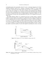
Pure HCF With LCF cracks
Figure 3.16. Comparison of number of cycles in last loading block of step test for HCF with and without LCF
precrack.
uncracked specimen. This observation is similar to the speculation in Chapter 2 where
tests at negative R are thought to initiate cracks at stresses below the failure stress when
using step loading.
Additional data are available on the number of cycles on the last loading block in the
step-loading tests when a crack is present. The data of Figure 3.16 are supplemented
with additional data on precracked notch specimens and replotted in Figure 3.17 as
a function of crack size. While very small crack lengths did not show a very well
0 × 10
0
2 × 10
6
4 × 10
6
6 × 10
6
8 × 10
6
1 × 10
7

0 100 200 300 400 500 600
Ti-6Al-4V
10
7
cycle blocks
K
t
= 2.2 notch
Last block cycles
Crack depth (microns)
Figure 3.17. Number of cycles in last block for notched bars with LCF cracks.
Accelerated Test Techniques 87
0 × 10
0
5 × 10
5
1 × 10
6
1.5 × 10
6
2 × 10
6
0 50 100 150 200
Ti-6Al-4V
2 × 10
6
cycle blocks
C specimen
Last block cycles
Crack depth (microns)

Figure 3.18. Number of cycles in last block for C-specimens with LCF cracks.
defined threshold, the longer crack lengths showed that specimens typically failed early
in the block, within a million cycles, indicating that the precrack eliminated some of
the initiation life. A similar observation can be made for the data in Figure 3.18 which
are obtained on a C-shaped specimen which was originally a pad in a fretting fatigue
experiment where cracks were formed on the pad in the contact region [31]. From
earlier observations, the HCF load block was reduced from 10
7
to 2 ×10
6
cycles. Here,
again, most of the failures occur within a million cycles, indicating that initiation life
in the step tests is reduced or eliminated. Of significance is the observation that in
both series of tests, uncracked specimens failed at a random number of cycles up to
10
7
, which was the loading block used in the step tests in both cases for uncracked
specimens.
Another example of the small number of cycles in the last block of step testing can
be seen in the work by Caton [32] on commercially cast aluminum alloy W319. In
this material, porosity plays the role of initial defects and, in that work, is treated as
an initial crack. Experiments were performed on three solidification conditions referring
to average secondary dendrite arm spacing (SDAS) of approximately 23 m 70m and
100 m denoted by low, medium, and high, respectively. The step-loading technique
to determine the FLS involved increments that were typically under 10% of the pre-
vious step stress and each step was carried out to 10
8
cycles or until failure occurred.
The number of cycles in the last block is plotted in Figure 3.19 for the three material
solidification conditions. With the exception of one data point, the results show that the

failure occurs early in the last step, indicating that the threshold for crack extension
is quite well defined in this material and that the initiation phase occurred at lower
stresses than the final block. For a material with initial defects, there may be little
88 Introduction and Background
0 × 10
0
2 × 10
7
4 × 10
7
6 × 10
7
8 × 10
7
1 × 10
8
Low SDAS
Medium SDAS
High SDAS
Last block cycles
Figure 3.19. Number of cycles in last block for cast aluminum step-tested at 20 kHz to 10
8
cycles (data
from [32]).
or no initiation phase because defects that act like cracks are already present in the
material.
Finally, we examine the results of fatigue limit testing using conventional constant-
stress testing. Exploring the fatigue limit corresponding to 10
9
cycles in a 1.8 kHz testing

machine, fatigue life and run-out data [33] are shown in Figure 3.20. It appears that
there is a small degree of scatter in the data, but the fatigue limit at 10
9
cycles can be
established as approximately 1020 MPa. It remains to be shown if a similar number can
be obtained using the step-test method using fewer specimens.
10
5
950
1000
1050
1100
10
6
10
7
10
5
10
9
10
10
Failure
Run-out
Maximum stress (MPa)
Number of cycles
1800 Hz
R = 0.8
Figure 3.20. S–N data for establishing N
f

at 10
9
cycles.
Accelerated Test Techniques 89
3.3.5. Comments on step testing
The results obtained on Ti-6Al-4V do not provide any conclusive evidence of a coaxing
effect. On smooth bar specimens and ones with carefully machined notches, the fatigue
limit is expected to have a small amount of scatter. The experimental data show this
in general, but the occasional data point which is higher than expected can either be
attributed to scatter or to coaxing. A systematic study of coaxing has not been conducted,
but up to this point the step-loading procedure appears to be a valid method which saves
considerable testing time. For specimens which have damage from FOD or fretting fatigue,
the statistical scatter is expected to be much larger. Whether or not high values of a FLS
are due to scatter or coaxing remains a question that may never be answered. Fortunately,
in design, an engineer does not have to worry too much about the occasional high value
of the fatigue limit, but rather the low ones and the range of experimental scatter. For
these purposes, a step-loading technique appears adequate for use on Ti-6Al-4V in both
bar and plate form. Its validity for use on other materials is yet to be established.
Another way to present data from step testing is illustrated in Figure 3.21 where, in the
test series, most of the tests had failures during the first step. Thus, what started out as a
planned step test series to evaluate the fatigue limit became largely an S–N test program.
Nonetheless, four tests reached the second loading block of 10
7
cycles and the run-out
data are shown with horizontal arrows. The data points for cycles on the last block are
also plotted. In this test series, the step sizes for the four step tests ranged from 11 to
19%, somewhat higher than what has been recommended. The first set of data points,
labeled “No step data” are conventional S–N data that could be extrapolated to longer
lives to estimate a FLS corresponding to 10
7

cycles. Such a value would appear to be
somewhat below 110 ksi as seen in the figure. No attempt was made to obtain a specific
10
4
10
5
10
6
10
7
10
8
90
100
110
120
130
140
150
No step data
Step data
Run-out
Step interpolated
Cycles to failure
Maximum stress (ksi)
PWA 1484
1100 F
R
= 0.1
Figure 3.21. Experimental data on PWA 1484 from step test series.

90 Introduction and Background
value because of the limited amount of data, particularly in the longer life region. The
next set of data points, denoted as “Step data,” are experimental values of the cycles
to failure in the last loading block of the step tests plotted against the stress that was
used in that block. In all four cases, the number of cycles represents that obtained in the
second block. Because of the large step sizes, one might be tempted to use these values
under the assumption that no history effect is present from the first loading block. This
turns out to be a very questionable assumption since failures occurred in other samples
tested at the same stress level as in the first loading block. These stress levels can be
seen from the data plotted as run-outs. These represent the first loading block of the step
tests and, in a conventional S–N testing program, would be the censored run-out data.
Arrows have been added to help identify the points which all correspond to a fatigue
limit of 10
7
cycles. Looking at these data combined with the “No step data” leads one
to revise the estimate for the FLS because there are now 3 run-out points at or above
110 ksi. Dealing with such limited data sets, the conclusion that there is a lot of scatter
in the FLS of this material starts to become more of a reality. Finally, we look at the
four interpolated points as computed from the step-testing procedure described earlier.
These seem to show that the fatigue limit is in the range 110–120 ksi. The above data set,
albeit quite limited, also shows some aspects of what has been interpreted as a coaxing
effect. The data points from the last cycle block in the step tests seem to lie above the
remaining S–N data, assuming that the first block of loading did no damage. A better
way to interpret these points is that they are from a censored set of samples, those that
did not fail during the first loading block. This simple data set and the various methods
of estimating the FLS serve to illustrate some of the complex issues that arise in trying to
determine FLSs from experimental data, especially when the number of available samples
or tests is quite limited and run-out data are involved. This subject is discussed in more
detail later in this chapter.
3.4. STAIRCASE TESTING

In addition to their statistical studies of number of cycles to fracture at each of a number
of stress levels, Ransom and Mehl [8] introduced a new abbreviated statistical method
known as “staircase testing.” which is still widely used today. In a series of tests, the
stress level for the next test is determined by whether the previous specimen failed or
ran unbroken for 10
7
cycles (survived). If the specimen failed, the stress on the next test
is reduced by one step. If the specimen survived, the stress on the subsequent specimen
is raised by one step, and so on. Statistical methods, described below, are then used to
determine the average endurance limit as well as the standard deviation. The results of
such tests on an SAE 4340 steel are shown in Figure 3.22 which includes the values of
the mean stress, 
0
, and the range ±2 where 95% of the values would fall.
Accelerated Test Techniques 91
40
42
44
46
48
50
52
54
56
10 20 30 40 50 60
Failure
Non-failure
Stress (ksi)
Specimen number
95%

s
0

=

46,270
s
0

+

2σ

=

52,080
s
0
–

2σ

=

40,460
0
Figure 3.22. Results of staircase testing on an SAE 4340 steel. Data are taken from [8].
The staircase method involves conducting a series of tests to a predetermined number of
cycles corresponding to what is defined as the FLS. The cycle count (often 10
7

cycles or
less) is assumed to be large enough to produce an endurance limit, but data show that
an endurance limit may not exist for most materials. Nonetheless, the FLS is a useful
number for many applications, particularly when the cycle count exceeds the number
of cycles that may be reasonably expected in the lifetime of a given application. In the
staircase method, the stress increment from one test to another is kept a constant.
∗
3.4.1. Probability plots
At the end of the up-and-down method, there are data at each stress level that was reached
which contain either failures or run-outs. Thus, for each stress level, the test data can
be used to calculate the percent of tests in which failure occurred. These data are used,
in turn, to compute a mean stress level at which 50% fail, 50% survive (run-out) and a
standard deviation about the mean. Some of the earliest data on the statistical nature of
FLSs, or endurance limits, were presented by Epremian and Mehl [9]. Based on a limited
number of staircase tests, the data shown in Figure 3.23 were obtained. They are plotted
on a linear scale as percent failures against stress for SAE 1050 steel. This type of plot
shows the cumulative distribution of percent failures for discrete values of stress level as
used in the staircase tests. If, as was done at the time, a normal distribution is assumed,
then a probability plot will produce a straight line as is illustrated for the same data in
∗
The staircase method was referred to as the “up-and-down” method in the early days of its development and
usage.
92 Introduction and Background
0
20
40
60
80
100
36 38 40 42 44 46

Percent failures
Stress (ksi)
Epremian and Mehl
(1952)
Figure 3.23. Experimental data of Epremian and Mehl on SAE 1050 steel [9].
39.5
40
40.5
41
41.5
42
42.5
43
.01 .1 1 5 10 20 30 50 70 80 90 95 99 99.9 99.99
Stress (ksi)
Percent failures
s = mean
Epremian and Mehl
(1952)
Figure 3.24. Probability plot of data from Epremian and Mehl [9].
Figure 3.24. On the probability plot, the mean value, ¯s corresponds to the intersection at
50% failures (40.8 ksi), and the slope of the line is a measure of the standard deviation.
If ¯s is the mean endurance limit and  is the standard deviation ( =1028ksi), then
¯s ±2 includes 95% of the endurance stress range.
Other examples of data from staircase tests can be used to illustrate the nature of the
probability plot used to estimate the mean of the distribution function and the ability of a
normal distribution function to represent the data. The results from Ransom and Mehl [8]
are plotted on a linear scale in Figure 3.25 and on probability paper in Figure 3.26. These
results are derived from a total of 54 tests, where equal numbers of failed and surviving
Accelerated Test Techniques 93

0
20
40
60
80
100
40 42 44 46 48 50
Percent failures
Stress (ksi)
Ransom and Mehl
(1949)
Figure 3.25. Experimental data of Ransom and Mehl [8].
44.5
45
45.5
46
46.5
47
47.5
48
48.5
.01 .1 1 5 10 20 30 50 70 80 90 95 99 99.9 99.99
Stress (ksi)
Percent failures
s = mean
Ransom and Mehl
(1949)
Figure 3.26. Probability plot of data from Ransom and Mehl [8].
specimens were obtained (27 each). Figure 3.25 shows that a simple distribution function
would not be able to represent these data to any reasonable extent. The plot includes the

stress level at which all of the specimens failed in the staircase testing, even though this
number is of little statistical significance. Continuing, however, with a probability plot,
Figure 3.26, an estimate of the mean is obtained as the intersection of the best-fit curve
(linear) with the 50% probability of failure line.
Similar plots are made from the results of 26 staircase tests on Ti-6Al-4V at a frequency
of 900 Hz and a stress ratio R = 01 [24]. The linear plot, Figure 3.27, shows that a
distribution function might represent this data set. Included in the plot, as done above
94 Introduction and Background
0
20
40
60
80
100
65 70 75 80 85 90
Percent failures
Stress (ksi)
Ti-6Al-4V
R
= 0.1
Figure 3.27. Experimental data on Ti-6Al-4V from National HCF program.
for the Ransom and Mehl data, are the stress levels where either none or all of the
samples failed. The probability plot for the titanium data is presented in Figure 3.28.
The limited data show that a straight line, representing a normal distribution, fits data at
the four stress levels where both failures and survivals occurred reasonably well. Two
additional data points, shown as circles, represent stress levels where either all or none of
the specimens failed. Assigning a probability of 99.9 and 0.1 to these stress levels shows
that these would not correspond to a normal distribution. Because there are so few data
at the extremes of stresses used in the staircase method, trying to estimate the tails of a
normal distribution curve is nearly impossible.

65
70
75
80
85
90
.01 .1 1 5 10 20 30 50 70 80 90 95 99 99.9 99.99
Stress (ksi)
Percent failures
s = mean
Ti-6Al-4V
R = 0.1
Figure 3.28. Probability plot of data on Ti-6Al-4V from National HCF program.
Accelerated Test Techniques 95
3.4.2. Statistical analysis
Data from staircase tests can be analyzed statistically by assuming any type of statistical
distribution for the percent failure data. Normal and Weibull distributions are the most
commonly used, but lognormal and smallest extreme value (SEV) distributions are also
found to be useful. If the stress increments are not constant, or data are obtained at lives
beyond the defined life used for the endurance limit definition (10
7
, for example) then
statistical analysis of the data becomes more complicated and other methods have to be
introduced [34]. An example of such data can be found in the final report on the National
HCF Program [24] where staircase tests, using 10
7
as the reference, often continued
beyond that cycle count because there was no automatic shutoff at 10
7
cycles if failure

did not occur when tests ran over a weekend or holiday.
For a limited set of data, the staircase method provides nearly the same value of the
endurance limit as regular S–N tests at constant stress levels. For a very large number
of tests, however, at many different stress levels in S–N testing, the S–N approach
provides more information about the dispersion of the endurance limit than the staircase
test method because fewer tests are conducted at the extremes of stress in the staircase
method. In the staircase method, it is assumed that the endurance limit is a statistical
variable. What is quite surprising is that, over the years, the endurance limit has often
been treated as a material constant. Epremian and Mehl [19], in 1952, noted, “It has been
known for some time that the fatigue life of a metal at a given stress varies statistically
and more recently it was discovered, in this laboratory,
∗
that the endurance limit is also
a statistical quantity and not an exact value.”
3.4.2.1. Dixon and Mood method
The statistics of the staircase method can be found in the paper by Dixon and Mood [35].
The staircase method, or the “up-and-down” method, is sometimes referred to as the
Dixon and Mood method and was developed for explosives research where an explosive
is dropped from a certain height and it either explodes or survives. This is an example of
an “all or none” philosophy that has been applied to the determination of fatigue limits
corresponding to a fixed number of cycles, 10
7
, for example. The primary advantage
of this method is that it automatically concentrates all of the testing near the mean.
As opposed to testing equal numbers of specimens at various levels, the up-and-down
method may save of the order of 30–40% in the number of observations [35]. Another
great advantage to the method is that the statistical analysis is quite simple under certain
conditions.
Many advances in statistical analysis of data come from the field of biology. In the book
by Finney [36], for example, the statistics dealing with the effectiveness of insecticides

∗
Carnegie Institute of Technology.