High Cycle Fatigue: A Mechanics of Materials Perspective part 14 docx

116 Introduction and Background
predictions, the RFL model, described above, was used. The baseline tests with N
f
< 10
6
cycles were selected as LCF tests that would typically be available from test programs
in addition to HCF properties. The RFL model treats run-out and failure tests with 2D
scatter in both life (LCF regime) and the endurance stress (HCF regime). An advantage
of the RFL model is that the 1D scatter assumptions are not required. The RFL model
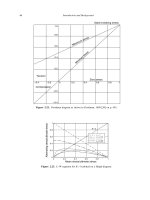
predictions with the baseline + step or staircase results are given in Figure 3.35.
If only the step tests are used in combination with the LCF tests, a tighter fatigue limit
variation is obtained with more error in life than for the staircase plus LCF tests where
fatigue limit variation dominates the life error term. In Figure 3.36, the average and lower
bound HCF limits for all approaches are summarized. If a 1D scatter in stress (s) is used,
similar lower bound predictions are obtained for the step and staircase tests. However, a
1D scatter in life results in a different lower bound as noted before. For the cases using
(a)
60
70
80
90
100
10
3
10
4
10
5
10
6
10

7
10
8
10
9
Baseline + step at interpolated S
max
S
max
(ksi)
Cycles
130
120
110
10% 50% 90%
Tighter fatigue limit
variation and higher life
error term vs staircase
(b)
60
70
80
90
100
10
3
10
4
10
5

10
6
10
7
10
8
10
9
Baseline + staircase tests
S
max
(ksi)
Cycles
130
120
110
10%
50%
90%
Fatigue limit variation
dominates life error term
Figure 3.35. Random fatigue limit model predictions using baseline tests (N
f
< 10
6
cycles) +step or staircase
approaches.
Accelerated Test Techniques 117
HCF Limits for Ti-6Al-4V at 75 °F and R = 0.1
40.0

60.0
80.0
100.0
Step
(s scatter)

Staircase
(s scatter)
Staircase
(N

f
scatter)
N

f
<

106
LCF
+ step
N

f
<

106
LCF
+
staircase

All BAA
single load
data
S
max
(ks)
average S
max
(ksi)
lower bound S
max
(ksi)
Analysis with 2D scatterAnalysis with 1D scatter
Figure 3.36. Summary of predicted average and lower bound HCF limits for Ti-6Al-4V at 75

F and R =01.
the 2D scatter, a similar lower bound is observed for either step, staircase, or all data,
when combined with the baseline LCF data. These predictions are seen to be different
than those obtained with the 1D scatter assumptions.
Another important feature that distinguishes the RFL model from conventional least
squares fitting (LSF) is the manner in which run-out tests are handled. As pointed out in
[50], the RFL model deals with the probabilities of an observation being above or below
some value whereas in ordinary LSF routines, the behavior is addressed as an average. In
the RFL model, each specimen has its own FLS. Least squares cannot deal with run-outs
because there is no specific data point to evaluate, but the RFL type model can deal
with the life exceeding some number at a given stress. These “censored” observations,
where a specimen could fail at any unknown time after the test was suspended, cannot
be included in any least squares calculations of the sum of the errors, so the LSF method
breaks down if these observations are to be included. For the RFL model, on the other
hand, these observations can be included if exceedance is the criterion being evaluated.

In the estimation of the parameters for the RFL model, a maximum likelihood approach
is used. As Annis and Griffiths [50] point out, if there are no censored observations, the
maximum likelihood method produces the exact same results as the least squares error
method.
As observed in all of the statistical approaches discussed above, and illustrated for
specific cases in Figure 3.36, the average HCF limits are relatively insensitive to the
assumptions. However, predicted lower bound limits are highly dependent on the assumed
scatter direction for the 1D scatter approaches (stress versus life scatter). Lower bound
limits are also highly dependent on the assumed scatter type (1D versus 2D scatter). In
the final report [24], the authors who represent the turbine engine industry conclude that
“the best approach needs to be assessed within the current design systems. Additional
work establishing confidence limits for the RFL model also is needed for use in design.”
118 Introduction and Background
The RFL assessment for all single load Ti-6Al-4V tests is also included as a final
assessment [24]. Load control tests with maximum stresses above the material yield stress
were not used in the final analysis. The model was fit with strain and load control tests at
different values of R with the 
equiv
damage parameter defined in Equation (3.20) below
as the alternating Walker equivalent stress and  is the total strain range for the cases
where inelastic behavior was encountered. 
max
is the maximum stress as measured on
test specimens or calculated with elastic-plastic analyses, and w is a material constant.
Strain control tests were used to establish the baseline half-life stress-strain properties. The
values of maximum stresses and strain were taken from strain control measurements near
the specimen half-life. The constant w =042 was obtained with a non-linear regression
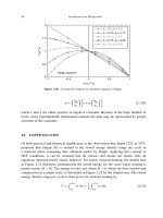
of the strain and load control tests. The average and −3s RFL fits are given in Figure 3.37.
The equations for the average and lower bound fit to the RFL model are:
Average fit: log N

f
 =−239472 log
equiv
−36199 +7629937 (3.16)
−3 fit log N
f
 =−239472 log
equiv
−23758 +7629937 (3.17)
In the RFL model development and analysis described in the section above, a SWT
and a 
equiv
parameter are used to consolidate data obtained at various stress ratios in
order to provide a larger database. The vertical axis in Figure 3.31 is the SWT parameter
while Figure 3.37 uses the 
equiv
parameter. The Smith–Watson–Topper [51] parameter
is defined as
SWT =


max
E
2

05
(3.18)
Ti 64 single load tests at 75 F (w = 0.42)
20
30

40
50
60
70
80
90
1.E
+ 03 1.E + 04 1.E + 05 1.E + 06 1.E + 07 1.E + 08 1.E + 09
Cycles
σ
equiv
(Ksi)
0.99
0.5
0.00135
Failures
Runouts
Figure 3.37. Single load test results and random fatigue limit fits for Ti-6Al-4V.
Accelerated Test Techniques 119
where 
max
is the maximum value of stress,  is the strain range, and E is Young’s
modulus. For purely elastic behavior, typical of the HCF regime, the formula becomes
SWT =


max

2


05
=
max

1−R
2

05
(3.19)
where R is the stress ratio. A modified version of the SWT parameter, used in industry
[52], has additional flexibility to consolidate data at different values of R. One form of
this modified parameter, which will be denoted as SWT
MOD
is
SWT
MOD
=05
w


max

1−w
(3.20)
where w is a fitting parameter. This modified version of the SWT parameter is often
referred to as an equivalent stress, 
equiv
. Equation (3.20) is written for purely elastic
behavior using  instead of E for the more general inelastic case. For the case where
w = 05, SWT and SWT

MOD
differ by a constant factor of
√
2 for all values of R. For
other values of w, the difference depends on stress ratio, R. Figure 3.38 shows values of
SWT and SWT
MOD
as a function of R for values of w =075, 0.5 and 0.25 to illustrate
the differences between the parameters. The values of the SWT and SWT
MOD
parameters
are normalized with respect to 
max
in the plots.
Step tests at the interpolated failure stresses were not used in the final baseline fits. Yet
for all of the other data, one observation still puzzles those involved in analyzing the data
obtained on Ti-6Al-4V. Though step and single load tests produced equivalent results
for R =01, step tests potentially produced unrealistically high allowable HCF limits at
R =−1, leading some to speculate whether coaxing actually exists in this material. In
their final report [24], the researchers recommended that “possible issues with step tests
at negative R should be assessed in future work.”
0
0.2
0.4
0.6
0.8
1
–1 –0.5 0 0.5 1
SWT
MOD (w

=

0.75)
MOD (w

=

0.5)
MOD (w

=

0.25)
SWT/
σ
max
Stress ratio, R
Figure 3.38. Normalized SWT and modified SWT parameter as function of stress ratio.
120 Introduction and Background
3.7. SUMMARY COMMENTS ON FLS STATISTICS
In summary, determination of the FLS and the corresponding statistics of scatter can
be accomplished in a number of ways. For the Ti-6Al-4V used in the National HCF
program, a number of methods and combinations thereof were used. The simplest case
was the use of step tests to determine the FLS by averaging the results of 5 tests. Next,
26 staircase tests were conducted and the results analyzed using the Dixon and Mood
method assuming a Gaussian distribution for the FLS. Third, results of a large number
of LCF tests including run-outs as well as a few long life tests beyond 10
7
cycles were

used in an assessment of the RFL model which considers scatter in both stress and life.
Finally, the RFL model was applied to a combination of the LCF data and the staircase
test data, where cycles to failure in the failed staircase tests were used as part of the
database. A summary of the results from the four procedures is presented in Table 3.9.
All data are presented for the FLS at 10
7
cycles and R =01. For the normal distribution
function, the −3 value is calculated. For the RFL model using the SEV distribution,
the value corresponding to a probability of failure of p = 001 at 10
7
cycles is used.
The results demonstrate that from four different combinations of databases and statistical
procedures that a mean value is obtained that has little variability among the procedures.
However, a design value at the tail end of a distribution function corresponding to −3
or p = 0001
∗
can have a large amount of scatter among the various techniques. It is
certainly not apparent what is the appropriate value of a FLS for design if the design
criterion is a probability of failure of one in a hundred or one in a thousand. It is not
even apparent what is the appropriate distribution function with which to represent FLS
based on sample sizes that do not exceed approximately 100. Another point to consider
in looking at the results presented in Table 3.9 is that the database used in the evaluations
with the RFL model contain data obtained at several values of stress ratio, R, while the
step tests and staircase tests were all performed at a single value of R. The RFL results
Table 3.9. Summary of statistical representation of FLS at 10
7
cycles, R =01
Data source Parameter Distribution
function
Mean

stress (ksi)
−3 value
(ksi)
Step tests FLS Normal 79.8 N/A
Staircase FLS Normal 78.0 51.1
LCF + HCF SWT SEV 80.3 601
∗
All (no step) 
equiv
SEV 79.5 535
∗
∗
Represents p =001 value in distribution function.
∗
For a normal distribution, a probability of failure of 0.001 corresponds to −3090. Conversely, −3
corresponds to p =000135. Similarly, p = 001 equates to −2326 while −2 equates to p =00227.
Accelerated Test Techniques 121
are interpolated for R =01 using the SWT or 
equiv
parameters. The scatter in the results
reflects both the inherent material variability as well as any inability of the models to
consolidate data at various values of R into a single parameter.
Another example of the possible problems that may be encountered in step testing,
in addition to those mentioned above for Ti-6Al-4V at R =−1, are associated with
data obtained on Ti-17 under the National High Cycle Fatigue program [24]. A limited
number of tests were conducted on this alloy at two stress ratios, R = 01 and R =−1.
Both conventional S–N tests, using single specimens at fixed stress levels, and step
tests where the specimen is reused until it fails, were conducted. The test matrix did
not constitute a statistically designed experiment, but the data obtained revealed some
interesting features. At R =01, Figure 3.39, S–N tests showed failures at stresses above

approximately 105 ksi and run-outs at stresses below that. Yet step tests produced slightly
higher values of the FLS at 10
7
cycles, with one test starting at 110 ksi and not failing on
the first block at that stress level where other samples had failed at cycle counts below
10
5
cycles. This anomalous behavior was attributed to a combination of material scatter,
possible variances in batches of material preparation/machining, and the possibility of a
coaxing phenomenon in this material. Even more perplexing are the results obtained at
R =−1 shown in Figure 3.40. Here, a similar phenomenon is observed as in the tests
at R = 01, but the number of specimens and the extent of the phenomenon seems to
be more prominent. While speculation abounded about the specimens coming from two
distinct batches that were prepared differently, no such conclusion could be drawn based
on incomplete records of the history of the individual specimens. The data, however,
seem to imply that there are two populations of specimens producing two distinct sets of
behavior. While the duality in S–N curves has been observed in gigacycle fatigue and
60
70
80
90
100
110
120
130
10
4
10
5
10

6
10
7
10
8
S –N tests
S –N run-out
Step run-out
Step tests
σ
max
(ksi)
N
Ti-17
R
= 0.1
350 Hz
Figure 3.39. Fatigue data for Ti-17 at R =01.
122 Introduction and Background
50
60
70
80
90
100
10
4
10
5
10

6
10
7
10
8
10
9
S –N tests
S –N run-out
Step run-out
Step tests
σ
max
(ksi)
N
Ti-17
R
= –1
350 Hz
Figure 3.40. Fatigue data for Ti-17 at R =−10.
has been associated with internal initiations at long lives, and surface initiations at shorter
lives in individual specimens,
∗
there were no internal initiations observed in any of the
specimens inspected after failure in the longer life (or higher strength) population of the
test results.
Another observation that is somewhat puzzling has been made in reviewing HCF limit
stress data on titanium. As seen in Figure 2.36 in Chapter 2 as an example, limited data
show an unusual amount of scatter for tests conducted at R =−1, fully reversed loading,
corresponding to zero mean stress. Bellows et al. [26] noted that the scatter in both step

tests and conventional tests was highest at R =−1. In addition to this being their only
test that went into compression, comparison with their other tests showed that these tests
had the highest stress (or strain) range and had the lowest value of maximum stress. No
readily observable differences were seen between the fracture surfaces of the step tests
and conventional tests at the same stress ratio.
The question remains as to whether fatigue lives at stresses above the fatigue limit
(infinite life) provide any information about the FLS or the FLS corresponding to a large
but finite number of cycles. Inherent in this discussion has to be the question about the
exact shape of the S–N curve and the extrapolation of this curve to large numbers of
cycles or to infinite life. Added difficulties arise from a statistics point of view because
the distribution function of lives at stresses producing finite lives and of fatigue limit
strengths at long lives or even at the fatigue limit for infinite life have to be known. An
evaluation of some aspects of this problem was made by Loren [53], who compared two
∗
See discussion in Chapter 2.
Accelerated Test Techniques 123
models for obtaining information on the fatigue limit (infinite life) and the endurance
limit defined as the fatigue strength at a given (long) life. The models were evaluated
based on numerical simulations of a staircase test procedure. For the fatigue limit model,
he assumed the fatigue limit is a random variable having a normal distribution of the
logarithm of the stress. If stresses are below the fatigue limit, they have infinite lives. In
the second model, the endurance limit (fatigue strength corresponding to a given number
of cycles) also is a random variable with a normal distribution of logarithm of stress. If
a specimen does not fail at a stress below the endurance limit, it has a life greater than
the cycle count at which the staircase testing is terminated. The lives are greater than
this cycle count, but not necessarily infinite. A large number of numerical simulations of
staircase testing were conducted corresponding to the statistical distribution assumptions
for each model. The results were analyzed using maximum likelihood procedures that
consider both censored (run-outs) and uncensored (failures) data. Both methods show that
it is possible to estimate the distribution of the fatigue limit, but the fatigue limit itself is

impossible to observe. The finite lives were found to give additional information on the
fatigue limit or the endurance limit in some cases, while in others they simply confirm
that the lives are finite. The results depend on the distribution functions as well as on the
life where the staircase tests are terminated. The statistical mathematics for conducting
these simulations are presented in the paper [53].
3.8. CONSTANT STRESS TESTS
If step or staircase tests are not used to provide information about the fatigue limit, tests
at constant stress levels can be used to determine the shape of the S–N curve. This is
particularly useful for LCF where the cycle counts are lower than in HCF. However, as the
S–N curve becomes more horizontal near the fatigue limit, the scatter in lives increases.
The choice of test method depends on, among other factors, the accuracy desired on both
the mean and the variance, the number of available samples, and the test time available.
If constant stress level testing is chosen, the number of tests at each level, the specific
values of the stress levels, and the stress increment between test levels have to be chosen.
While guidelines exist for test planning purposes [54], they are very restrictive and pertain
only to S–N relationships that are linear on the proper coordinates, that variance in
fatigue life is the same at the various stress levels, and that there are no run-outs. For
optimum results on real data, the number of tests at each level does not have to be a
constant. Beretta et al. [55] conducted a very large number of tests on a 0.43% carbon
steel to establish the fatigue properties and scatter for the material. They then conducted
a statistical analysis to determine confidence levels of test sequences where the number
of tests at each stress level was not constant. The statistical analysis took into account
run-outs. As they point out, most existing recommendations are based on assumptions of
124 Introduction and Background
the lognormal distribution of lives, the absence of run-outs and, more restrictively, the
same variance at each stress level. In their work, they assumed a lognormal distribution
of lives at each stress level based on test results, but the distribution was different at
each stress level. The largest scatter, as expected, was at the lowest stress level. Three
statistical models were considered which have different relationships between the standard
deviation and the applied log-stress: exponentially variable according to an exponential

model by Nelson [56], linearly variable, and constant. The equations describing these
models are shown below. For the mean, , the three models use
 =X
1
+X
2

logS −
logS

(3.21)
while the three models use the following functions for :
 = exp

X
3
+X
4

logS −
logS

(3.22)
 = X
3
+X
4
logS −log S (3.23)
 = exp


X
3

(3.24)
where S is the applied stress,  is the mean value and  is the standard deviation of the
(log) fatigue life, while
logS is the arithmetic average of all the values of log S in the test
series. The constants X
1
X
2
X
3
, and X
4
are fitting parameters for each statistical model
based on maximum likelihood estimates. While the same function, Equation (3.21), is
used for the mean, , for each of the models, the values of the parameters X
1
and X
2
are slightly different for each model because of the different distribution functions which
they represent.
Using maximum likelihood analysis on the results of fatigue tests they obtained on the
0.43% carbon steel including run-outs, the parameters in the equations were determined
for the three models. The models are shown, without the experimental data, in Figure 3.41
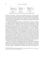
(a) through (c) where the mean (50% probability of failure) and 2.5 and 97.5% probability
of failure curves are shown for each of the models. The differences in the distributions
can be clearly seen, particularly at the lower stress levels.
To evaluate the results of using a small sample size, confidence levels were determined

for various sample sizes randomly extracted from the total population of tests run for each
model. The first point noted was that the model using a constant standard deviation, ,
Equation (3.24), independent of stress level (Figure 3.41c), provided the worst fit to the
data and was not used in subsequent computations. It has been noted that the assumption
of constant  is the most commonly used, and virtually all statistical computer programs
for curve fitting make this assumption because the mathematical theory and numerical
computations are then simpler [56]. They observed that the Nelson model that uses the
exponential variation of  (Figure 3.41a) provides the best estimates of model parameters
Accelerated Test Techniques 125
400
500
10
4
10
5
10
6
10
7
Stress amplitude (MPa)
Cycles to failure
600
2.5%
50%
97.5%
(a)
10
4
10
5

10
6
10
7
400
500
Stress amplitude (MPa)
Cycles to failure
600
2.5%
50%
97.5%
(b)
400
500
10
4
10
5
10
6
10
7
Stress amplitude (MPa)
Cycles to failure
600
2.5%
50%
97.5%
(c)

Figure 3.41. Models for fatigue life with standard deviation a function of stress: (a) exponential (Nelson),
(b) linear, (c) constant.