High Cycle Fatigue: A Mechanics of Materials Perspective part 15 ppsx

126 Introduction and Background
and of mean log-lives for a material having variable scatter, provided that the precision
at the highest stress level is markedly lower than the others. Their results also showed
that results obtained from test programs with different number of specimens per level are
better than those of plans with uniform replication. For the particular set of data used, from
which experimental results were chosen at random for the statistical analysis, a confidence
level of 90% could be obtained over the range ± using the following test programs:
10–3–5–6 specimens (a total of 24 specimens) tested at levels 550–520–490–460 MPa
for the exponential (Nelson) model, Equation (3.22), and 10–3–6–10 specimens (a total
of 29 specimens) tested at the same stress levels for the linear model, Equation (3.23).
3.8.1. Run-outs and maximum likelihood (ML) methods
A unique feature of testing in the HCF regime is the occurrence of run-out tests where
the test is terminated after a certain (large) number of cycles. Alternately, a test that fails
after N cycles can be used in an analysis describing the behavior for fewer than N cycles,
so it can then be treated as a run-out for the fewer cycles being considered. Run-outs,
in statistics terms, are considered to be censored data, that is, they fall outside the range
of behavior (lives) being considered. In fitting models to data containing run-outs, the
run-outs cannot be used in least-square fits because the exact location of the data point
is unknown. All that is known is the fatigue life was greater than some quantity. Since
least-squares methods cannot use censored data because the data points do not really
exist, other methods have been employed. As mentioned in the discussion of the RFL
model previously, maximum likelihood (ML) estimation schemes are able to deal with
censored data from a statistical point of view. The virtue of the ML method is that it
applies to virtually any assumed statistical distribution of lives or fatigue strengths as well
as any form of data including run-outs. Details regarding ML theory and its application
to fatigue data, particularly in the HCF regime, can be found in the book by Nelson
[57], for example. The ML method not only provides valid estimates of the mean and
standard deviation of a distribution function, it also provides confidence intervals for
coefficients in the distributions or models. The application to various models for variable
standard deviation, , as a function of stress, for example, was discussed above. ML
estimates have good statistical properties for almost any assumed form of the fatigue

life distribution and for almost any assumed form for the equation for the distribution
parameters as functions of the stress or other variable [56]. In some simple cases where
fatigue life is described by a lognormal distribution with constant  and there are no
run-outs, ML estimates of model coefficients are the same as standard least-squares
regression estimates. Although ML methods are mathematically complex, they are easy
to apply in practice using special computer packages that are now widely available [57].
The procedure involves writing equations for the likelihood of an event (failure in a
given lifetime, for example) in terms of the unknown parameters of the distribution
Accelerated Test Techniques 127
function and/or model. The values of the coefficients that maximize the likelihood are
then determined. This procedure generally involves nonlinear equations that cannot be
solved algebraically, thus numerical methods are employed. The solution of these types
of equations is what statistical computer codes are designed to accomplish using various
numerical techniques. It is important that the solutions provide a global maximum of the
likelihood function, not a local maximum nor a saddle point. Existence and uniqueness of
the solutions also have to be established. There are some models for which the likelihood
equations can be solved explicitly [57].
As a simple example of the ML method, we consider a set of ten hypothetical exper-
iments at constant stress where the log lives to failure from each test are tabulated in
ascending order in Table 3.10. These data are labeled “actual” and represent a data set
where all tests would have been carried out to failure.
If these same tests had been conducted up to 10
7
cycles (log life = 7) and terminated
at that point if no failure had occurred, then 3 of the tests would be recorded as run-outs
(censored). Both sets of data are shown in Figure 3.42 on a probability plot assuming
the log lives follow a normal distribution. The actual data are fit with a straight line to
determine the constants for the normal distribution that represents this data set.
If the same data are taken with run-outs, the data set including 3 censored points that
indicate only that the observed log lives were >7, the ML method can be employed.

Using a commercial software package called Minitab, the data were evaluated assuming
a normal fit to log life as was the case for the real data [58]. The results of that evaluation
are shown in Figure 3.43 which shows both the best fit to a normal distribution of log
life (time) as well as the 95% confidence bounds. The fit is almost identical to that of
the entire (uncensored) data set shown in Figure 3.42.
For comparison purposes, the results of both fits are presented in Table 3.11. The
analyses show that the ML method, using 7 data points and 3 run-outs, produces essentially
Table 3.10. Hypothetical log
life data for testing with and
without run-outs
Actual Censored
5.8 5.8
6.0 6.0
6.2 6.2
6.3 6.3
6.5 6.5
6.7 6.7
6.9 6.9
7.1 7 run-out
7.3 7 run-out
7.6 7 run-out
128 Introduction and Background
5 5.5 6 6.5 7 7.5 8
.01
.1
1
5
10
20
30

50
70
80
90
95
99
99.9
99.99
Log cycles
Percent
Censored
Actual
Figure 3.42. Statistical distribution of lives to failure with and without run-outs.
98765
99
95
90
80
70
60
50
40
30
20
10
5
1
Time to failure
Percent
Figure 3.43. Statistical analysis of censored data using ML method.

Table 3.11. Constants for normal distribution of log life
from standard and ML methods
Actual Censored
Mean Stdev Mean Stdev
6.640 0.585 6.644 0.571
Accelerated Test Techniques 129
the same normal distribution as standard least squares methods for the specific data set
of 10 data points chosen for this numerical example.
3.9. RESONANCE TESTING TECHNIQUES
Structural components subjected to high frequency vibrations, such as those used in
rotating parts of gas turbine engines, are usually required to be designed using a lifetime
failure-free criterion for a very large number of cycles, or an endurance limit. Tools, such
as the constant life Haigh or Goodman diagram, described earlier in Chapter 2, are often
used, but these diagrams are usually constructed using uniaxial fatigue data only, and the
design is based on uniaxial stresses. While it is desirable to have data at many values of
mean stress, or equivalent stress ratio, R, there are many cases in design where data at a
single value of R =−1, fully reversed loading with zero mean stress, are the only data
available. Such data, often obtained from vibratory tests on a specimen or component, are
then used to construct a Modified Goodman diagram using a straight line extrapolation
from the zero mean stress data point to the yield or ultimate strength of the material
which is considered as zero alternating stress (see Figure 2.17 in Chapter 2). Alternate
approaches such as the Jasper or other equation, as described earlier, can be used to
construct a Haigh diagram by using an equation to represent behavior at all values of
mean stress or stress ratio, but data for at least one value of R are needed to establish the
constants.
Uniaxial fatigue tests on conventional test machines are the type of test normally
conducted to obtain the required data for construction of a Haigh diagram. These tests
require long time periods to achieve a large number of cycles approaching the endurance
limit. Even a servo-hydraulic test machine operating at 60 Hz requires approximately
46 hours to accumulate 10

7
cycles for a point on an S–N curve. Additionally, for
each value of mean stress or stress ratio, several data points are needed in order to
interpolate the value of stress at the desired life (10
7
in this example) to get a single point
on the Haigh diagram. Therefore, significant amounts of time are required to characterize
the uniaxial fatigue properties of a material. While newer machines are available which
can achieve higher frequencies, and ultrasonic machines that operate at 20 kHz have
been developed [2], these tests are typically limited to uniaxial tension. Accelerated test
methods, described in previous sections in this chapter, and test procedures such as step
or staircase testing, described above, can save some time. However, these provide only
uniaxial fatigue data which may be insufficient for assessing high cycle FLSs which
often occur in components that are subjected to biaxial loading over a wide range of
cyclic frequencies. In turbine blades, for example, fatigue failure often occurs under high
order bending or combined bending and twist modes that produce short wave length
stress states at very high frequencies. Unfortunately, the current capability to conduct
130 Introduction and Background
biaxial fatigue tests, especially under bending or torsion as well as axial stress states,
is limited by the high cost of development of such testing methods as well as the lack
of existing equipment to conduct the necessary tests at anything other than very low
frequencies.
Resonant fatigue testing of some unique geometric configurations has recently been
proposed [59] as a method for obtaining data heretofore unavailable because they involve
both high frequencies and either uniaxial or biaxial bending stress states. It should be
noted that resonant fatigue testing procedures have been in existence for over a century.
In reviewing the history of resonant techniques, it can be pointed out that in the time
period from 1879 to 1925, no fewer than 35 journal articles appeared describing new
test procedures and methods for fatigue testing [60]. The earliest test methods involved
coupling a specimen and a driver in order to obtain a resonance or near resonance condition

to decrease the power requirements. It was recognized early on that “working in or
near the resonance (unstable dynamic equilibrium) demands special controlling devices”
[61]. These early machines were only able to achieve frequencies up to approximately
100 Hz and were confined to either pure axial or torsion modes under either resonant
or non-resonant conditions [62]. Among the early test machines that operated on the
resonance principle were those built by Sontag that produced a constant force at 30 Hz.
The Schenck machines, of the 1930s and later [63], operated in a fairly stable manner by
using a very large spring coupled to a much smaller specimen and could run continuously
under constant load at approximately 30 Hz. Later on, such machines were controlled
with automatic feedback from a load cell to correct for any deformation of the specimen
during the test such as creep or initiation of a fatigue crack. A very large version of a
Schenck machine [64] was used in the Messerschmitt factory during World War II to test
large components, but the loading was still uniaxial. Electromagnetic resonant fatigue test
machines are currently available having high-test frequencies of 40–300 Hz and boast of
the same advantage of the first machines, namely low power consumption.
One of the advantages of a resonant machine where the specimen is part of the
mechanical system is that upon incipient failure, the spring constant of the specimen
changes and throws the system off resonance which is a warning of impending failure
if it is desired to examine the specimen before total destruction of the sample [65]. In
addition to mechanically driven machines, magnetic excitation to drive a machine/sample
combination into resonance dates back to prior to World War II (see, e.g. [66]).
Tests of structural components and full-scale structures conducted under both resonant
and non-resonant conditions [67] date back to the 1860s [68]. Because of the expense
of the test articles as well as the test machines, such tests are normally limited to very
few components and are not very useful for extracting fatigue properties of the material,
even though the stress state at a failure point may be complex. Whatever information is
extracted is limited to the specific number of cycles to failure due to the applied loading
Accelerated Test Techniques 131
condition. Fatigue limit strengths of the structure or the material are rarely obtained for
cycle numbers near the endurance limit.

As discussed earlier in this chapter, a step-test procedure has been shown to produce
fatigue limit data that are consistent with those obtained from interpolation of S–N
curves at fixed values of mean stress or stress ratio. With a limited number of samples,
since each sample produces a FLS data point, a Haigh diagram can be constructed
in a reasonable amount of time. To achieve the goal of determining the FLS under
uniaxial or biaxial bending, stress states that are commonly achieved in turbine blades
under resonance conditions, a combination of the concepts described above have been
utilized and expanded to develop a new testing procedure [59]. This vibration-based
fatigue testing concept uses a base-excited plate specimen that is driven into a high
frequency resonant mode. Using the step-testing procedure and finite element analysis
of the vibrating specimen, the loads and stresses necessary to produce HCF failure
corresponding to a fixed number of cycles (10
6
or 10
7
) can be determined. The geometry
of a plate that is driven into resonance by base excitation on a shaker can be either a
square plate for uniaxial bending or a more complicated geometry as shown in Figure 3.44
for biaxial bending. For a square plate of steel with dimensions of 114 mm on a side, the
natural frequency under a two-stripe mode is approximately 1200 Hz. The out-of-plane
displacement profile and corresponding vonMises stresses are shown in Figure 3.45 for
61.0
61.0
20.3
162.6
81.3
Clamped edge
35.6
50.8
Figure 3.44. Resonant biaxial specimen dimensions (mm).

132 Introduction and Background
(b)(a)
Figure 3.45. Out of plane displacements (a), and vonMises stresses (b), for square steel plate.
the steel plate of 2.4 mm thickness. The maximum stress occurs at the middle of the free
end (top of picture) and is higher than any stresses at the fixed end (bottom) which is
being excited by the shaker. The stresses at the free end were sufficient to cause cracks
to form within 10
6
cycles using a conventional laboratory shaker/amplifier system [59].
For biaxial loading, the specimen shown in Figure 3.44 was base excited into a resonant
two-stripe mode frequency of approximately 1600 Hz. The specimen was aluminum with
a thickness of 3.1 mm. The out-of-plane displacements and vonMises stresses for the
square steel and aluminum biaxial specimens are compared in Figures 3.45 and 3.46.
(a)
(b)
Figure 3.46. Out of plane displacements (a), and vonMises stresses (b), for aluminum biaxial specimen.
Accelerated Test Techniques 133
Figure 3.46 shows that the maximum stresses for the aluminum biaxial specimen occur
along the centerline and away from the free end by approximately one-third of the length.
For this particular geometry, the ratio of 
y
(vertical direction) to 
x
(horizontal direction)
at the point of maximum stress is approximately 0.59.
These specimen geometries and the resultant two-stripe mode shapes of interest have
been used to determine FLSs under uniaxial or biaxial bending with a step-test procedure.
The mode shapes that were predicted by finite element method (FEM) and verified
experimentally provided a method for calibrating stresses at the critical locations with
observed transverse displacement amplitudes recorded with a laser vibrometer.

The fatigue limit strength in typical uniaxial tension tests, performed using conventional
testing machines, is determined as the stress at which complete failure occurs under
constant load, either by conventional S–N or step testing. For long life tests, total life,
where the fatigue crack propagates through the specimen and failure occurs, is not
distinguished from crack nucleation or crack initiation life. Computations have shown
that the fatigue crack propagation life in a tensile bar is only a small fraction of total life
when testing at stress levels near the HCF limit defined as 10
7
cycles [69]. In the case
of vibration-based fatigue testing under resonance conditions, however, there does not
exist a definitive phenomenon such as abrupt failure. Therefore, in the vibration-based
tests, from the start of the test until the time of fatigue crack initiation, the response
amplitude of the plate as measured by a laser vibrometer has to be monitored and adjusted
by changing the amplitude and frequency of the shaker to keep the system in resonance
and to maintain the desired stress level. In this technique, the fatigue limit is defined at
the instant corresponding to a sudden change in the response of the plate, as opposed
to the typical gradual changes in the dynamic response of the plate associated with the
stiffness changes associated with fatigue crack development. A resonant frequency shift
away from the shaker driving frequency was observable even in the initial stage of fatigue
crack development [59].
In the tests conducted by George et al. [59], the vibration testing was continued in
one of two ways after the FLS was determined. By varying the experimental technique,
they were able to produce both short and long cracks. The technique to produce short
cracks, on the order of a few millimeters or less, was to leave the shaker amplitude fixed
after the FLS was determined and to propagate the crack by repeatedly re-tuning the
shaker driving frequency to the resonant specimen frequency. As the crack propagated,
the resonant frequency of the specimen decreased. With this technique, using a constant
shaker amplitude, the maximum stress level in the crack tip region ultimately dropped to
a level where the crack arrested. This technique produced cracks on the order of 1–2 mm
in the case of steel specimens and 0.1 mm in the case of Ti-6Al-4V. To produce long

cracks, on the order of tens of mm, the shaker amplitude had to be increased as necessary
to continue propagating the crack.
134 Introduction and Background
For the biaxial specimen of Figure 3.44, the frequency response exhibited nonlinear
hardening which produces specimen response at the natural frequency which is unstable
[59]. As the fatigue crack begins to develop and decrease the stiffness of the plate the
natural frequency begins to drop and the response immediately decreases drastically.
This sudden drop enables small cracks to initiate and then arrest because of the sudden
decrease in the forcing function. This phenomenon enabled George et al. [59] to produce
an approximately 0.4 mm long series of microcracks in their biaxial specimen.
One of the most important observations from the experiments of George et al. [59] is
that the formation of a crack in a specimen reduces the natural frequency of the system.
If the frequency of the excitation remains fixed, the level of response at that frequency
will be reduced, and a new peak response will be present at a lower frequency. This
observation in itself is not new, but its implication on gas turbine engine fatigue could
drastically change widely held design and maintenance conventions. From the fatigue
perspective, this implies that for a constant level and frequency of excitation, once a
crack is initiated, the level of strain in the component is reduced. If this level of strain is
reduced below the level needed to propagate the crack, the crack will self-arrest. In order
to continue crack growth, the frequency of excitation must be reduced to meet the new
peak response frequency, and if it does, the fatigue process continues. For the case of
forced response in a gas turbine engine, where the excitation consists of distinct tones, or
narrow bands, of aerodynamic drivers, a crack could self arrest once the peak response
frequency shifts away from the forcing frequency. For high order modes, where mode
shapes tend to have localized areas of high strain, a small crack might form, propagate
slightly and then arrest without having an adverse effect on the overall structure. For
a broadband excitation, such as inlet distortion or low order excitation of the turbine
from combustor effects, the above scenario is less likely and the crack would continue to
propagate since an excitation would be strong over a wide range of frequencies. As with
classic laboratory fatigue experiments in which a crack is chased by changing frequency

to continue crack propagation, as the natural frequency of the component changed, there
would be an excitation waiting to continue fatigue through to failure.
3.10. FREQUENCY EFFECTS
Questions have arisen over the years about frequency effects on the HCF behavior and
fatigue limit strength of materials and structural components. While laboratory testing
has traditionally dealt with frequencies typically below 100 Hz,
∗
components in turbine
engines can undergo vibratory stresses well into the kHz regime. It is natural to ask,
therefore, what effect does frequency have upon the fatigue behavior of materials. Dealing
∗
See Chapter 2, Section 2, for a discussion of gigacycle fatigue and testing at 20 kHz.
Accelerated Test Techniques 135
solely with material behavior, data on a number of structural materials [70], show that
metals exhibit very little difference in strength in terms of strain rate effects up to nominal
strain rates in the 1–100s
−1
regime. However, these rate effects are confined to the
inelastic regime of material behavior, so these numbers should not necessarily apply to
fatigue in the HCF regime where behavior is nominally elastic. Further, for the purpose
of translating strain rates into equivalent frequencies, consider that nominal maximum
strains in the HCF regime are of the order of less than 1% (0.01), so a frequency of 1 kHz
would correspond to a strain rate of less than 10 s
−1
. Finally, gigacycle fatigue testing
conducted at frequencies of 20 kHz has shown little or no difference in fatigue strength
than results obtained at conventional frequencies. It is significant to note that, for reasons
not related to frequency effects, gigacycle fatigue testing is being conducted by many on
rotating beam machines that operate at under 60Hz.
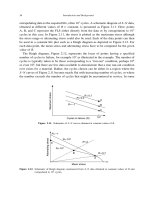
It is with great interest and curiosity that examination of the results of fatigue tests

conducted in the 1950s and earlier show what appear to be frequency effects in a number
of materials. Lomas et al. [71] summarize many of the findings up to their publication
date in 1956 which includes much speculation as to the validity of many of the early
results reporting frequency effects. Most of the data were considered unreliable and some
of the findings were attributed to heating effects at higher frequencies. They cite the
work of Jenkin [72] and Jenkin and Lehmann [73], the latter of who’s work they plot
in their paper, reproduced here as Figure 3.47. The materials represented here include
copper, aluminum, and several steels: 0.86% carbon, 0.11% carbon, rolled, Armco iron,
Copper
Aluminium
a
b
0.86% carbon
Armco iron
FREQUENCY-CYCLES PER SEC.
10,000
3,000
1,000
300
14
16
18
20
22
24
26
28
30
32
34

4
5
6
FATIGUE LIMIT-TONS PER SQ. IN.
0.11% carbon,
rolled
0.11% carbon,
normalized
Figure 3.47. Endurance stress data of [73] replotted by Lomas et al. [71].