High Cycle Fatigue: A Mechanics of Materials Perspective part 17 pptx

146 Effects of Damage on HCF Properties
Log stress, σ
Log flaw size, a
Threshold stress intensity, Kth
FATIGUE
REGIME
σ
e
Endurance limit stress, σ
e

Growth below long
crack threshold
Growth below
endurance limit
El Haddad a
0

correction
a
0
Figure 4.1. Schematic of a Kitagawa diagram.
should not grow.
∗
There are two regions shown in the diagram where cracks can exist
either below the endurance limit or the below the extrapolated long crack threshold. In
the first case, the crack behavior is dominated by fracture mechanics, not stress. In the
second, the small crack correction of El Haddad smoothes out the threshold curve in
order to meet the endurance limit at very small crack lengths.
The Kitagawa type diagram [2], shown again schematically in Figure 4.2, is a useful
tool to evaluate the potential for a crack to reduce the HCF capability of a material,

irrespective of crack size. This plot of stress  against crack length (a) on log–log
scales was first suggested for a simple edge-crack geometry where stress intensity is
proportional to
√
a. The endurance limit when no crack is present, or the threshold stress
intensity when there is a crack, represent the limits above which failure might occur
and below which it will not, corresponding to some chosen number of cycles or crack
growth rate, respectively. The endurance limit is a horizontal line in Figure 4.2 while
the threshold stress intensity is line of slope =−05 for the simple edge crack. The two
∗
The terminology for the diagram with log stress plotted against log crack length [2], used subsequently for
any crack geometry and stress ratio, is referred to variously in the literature as a Kitagawa–Takahashi diagram,
a K–T diagram, a Kitagawa type diagram, or most commonly, a Kitagawa diagram. In this book, the common
terminology “Kitagawa diagram” will be used to refer to that type of plot. In a similar manner, the terminology
“El Haddad short crack correction” will be used to represent the contribution of El Haddad et al. [3]. The use
of this terminology is in no way meant to be disrespectful to, or to ignore the contributions of, the co-authors of
Kitagawa or El Haddad in the referenced publications. Rather, the respective terminologies are for convenience
only.
LCF–HCF Interactions 147
Log stress, s
Log flaw size, a
Threshold stress intensity, K
th
Endurance limit stress, s
e
Short crack correction
a
a
0
a

0
Figure 4.2. Schematic of a Kitagawa diagram for any geometry. Short cracks of length a behave as if they
were long cracks with length a +a
0

lines can be connected to form a single curve for all crack lengths using the short crack
correction proposed by El Haddad et al. [3]. In the work of Moshier et al. [4], it is shown
how the Kitagawa diagram can be used for any crack geometry. In their application,
they applied it to a surface flaw in a double-edge-notch tension specimen. Of particular
significance in using the Kitagawa diagram for any geometry is that the endurance limit
and the value of a
0
for the short crack correction are not material constants but, rather,
material parameters for the particular geometry and stress ratio, R, being investigated.
To describe the Kitagawa diagram mathematically for any geometry, the following
analysis is presented. The K solution for any crack geometry can be written in the form
K = 
√
a Ya (4.1)
where K is the stress intensity,  is the stress, a is the crack length, and Ya defines
the K solution for a particular geometry. If Equation (4.1) is written for the threshold
condition of a long crack, and the crack length is represented by a
1
, then the long-crack
solution for stress as a function of crack length, the threshold line in Figure 4.2, is
 =
K
thLC
√
a

1
Ya
1

(4.2)
where K
thLC
represents the long-crack threshold stress intensity, a material constant for
a given stress ratio, R. Denoting the intersection of the long crack threshold and the
endurance limit stress in Figure 4.2 by a
0
, the intersection is defined in the equation

e
=
K
thLC
√
a
0
Ya
0

(4.3)
148 Effects of Damage on HCF Properties
where 
e
is the endurance limit stress for the particular geometry for which the K solution
is given by Equation (4.1). The usual form for this equation solves for a
0

,
a
0
=
1


K
thLC

e
Ya
0


2
(4.4)
and is commonly found with the Ya term missing or equal to a constant. For the more
general case, either of these Equations (4.3) or (4.4), can be solved for a
0
either iteratively
or graphically. Equation (4.4) for a
0
will be used extensively in the remainder of the book
and will be repeated quite often.
The short crack correction of El Haddad et al. [3], shown graphically in Figure 4.2,
uses the concept that a crack of length a behaves as if it had a length a +a
0
, which has
the long crack threshold value. Noting that the crack length a

1
can be written as
a
1
=a+a
0
(4.5)
the FLS for any true crack length a becomes, from Equations (4.2) and (4.5):
 =
K
thLC

a +a
0
 Ya +a
0

(4.6)
where, as the crack length goes to zero, the FLS goes to 
e
. The short crack curve in
the Kitagawa diagram is easily constructed if the long crack curve exists by taking the
value of a for any value of stress from Equation (4.2) and reducing it by a
0
. Alternately,
if the effective value of K is wanted for a short crack [5], it is easily shown that the
effective K is
K
thSC
=K

thLC

a
a +a
0
Ya
Ya +a
0

(4.7)
where, as in the calculation for a
0
, the Y terms can usually be ignored.
The significance of the Kitagawa diagram with the short crack correction is that it
shows, if the threshold data follow the curves, that cracks of length a
0
or less, have FLSs
which are not significantly lower than the endurance limit for a particular geometry. At
a crack length of a
0
, the FLS is 1/
√
2or071 of the endurance limit. If cracks are
formed at LCF stresses that are higher than the HCF limit, then the cracks that eventually
propagate under HCF may act as if an overload occurred which may retard the crack or
increase the fatigue limit [6]. Thus, it is not surprising to find that small cracks formed
under fretting fatigue [7], or under LCF at notches [8], or in smooth bars, do not have a
significant detrimental effect on the FLS. These cases are discussed later in this chapter.
LCF–HCF Interactions 149
4.1.1. Behavior of notched specimens

A Kitagawa type plot can be used to represent what happens in a notched bar, as has
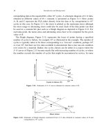
been done by Moshier et al. [4, 9]. A schematic of threshold stress as a function of
crack length, assuming no load-history effects in the crack growth behavior, is given in
Figure 4.3 for two different cases. The diagram shows two curves, an upper and a lower
one, which represent what is commonly termed blunt notch and sharp notch behavior,
respectively. Above or below each curve, there is either crack initiation and growth to
failure at higher stresses, or no initiation or growth at lower stresses, respectively. The
two curves represent the relation between stress and crack length corresponding to the
K-solution for a crack emanating from a notch. The solution is corrected for small crack
behavior as per the approach suggested by El Haddad et al. [3]. For the blunt notch case,
represented by the upper curve through A, a crack that forms will continue to propagate
because the stress for crack initiation or threshold crack growth is a decreasing function
of crack length. However, in region I below the curve, stresses are below the endurance
limit, and cracks should not form in this region unless the history of loading is such to
allow formation of a crack. The line through A in the diagram, which is constructed for
a specific notch geometry, is valid only for that geometry at a given stress ratio. Cracks
formed in region I must, therefore, form from some other loading condition. The point A
in the figure, which represents the endurance limit of the notched bar, is often taken to be
the smooth bar endurance limit stress, 
e
, divided by k
t
. Data such as those of Lanning
et al. [8] indicate that this is not necessarily the case for mildly notched titanium bars.
While the value of stress at A can be written as 
e
/k
f
, where k
f

is the fatigue notch
factor, this is no more than a mathematical definition of the endurance limit stress for
the notched body. The stress at A is not a material constant, but a geometry-dependent,
empirically determined quantity. The subject of fatigue thresholds for cracks at notches
is discussed in more detail in Chapter 5.
Log crack length, l
Log threshold stress
I
II
A
B
C
D
l
No crack growth
Crack growth
to failure
Figure 4.3. Schematic of a Kitagawa type diagram for notched specimens.
150 Effects of Damage on HCF Properties
A Kitagawa type diagram was used by Moshier et al. [4] for mildly notched specimens
which were precracked under LCF. The endurance limit stress for any crack length was
found to be well predicted by a load-history dependent model [6], described later in
this chapter, combined with the equations that connect the long crack threshold and the
notched specimen endurance stress using the small-crack correction from El Haddad
et al. [3]. It should be noted that the parameter a
0
used in the El Haddad correction,
is not a material constant when used for notches in the manner described here. Rather,
it represents the crack length where the long crack K solution for the notch, K = K
th

,
intersects the endurance limit given by the stress at point A in the diagram (Figure 4.3).
In region II of Figure 4.3, above the lower curve which represents the K solution for
a very sharp notch, typically one with a k
t
value in excess of approximately four or five,
cracks are known to be able to initiate but not continue to grow. Until the stress exceeds
the value at B, and for crack lengths below that indicated by point D, a crack may initiate
but arrest. As in the case described above, the stress above which cracks initiate, C,is
often taken to be 
e
/k
t
, but it is extremely difficult to verify this and, further, this value
is of minor engineering significance. What is of greater significance is the empirically
determined endurance stress, B, under which a specimen will both initiate a crack and
continue to propagate it to failure. Again, this endurance limit is not a material constant
but, rather, an empirically determined quantity that depends on the particular sharp notch
geometry. While cracks of lengths less than that of point D may initiate and arrest, these
crack lengths are generally very small (the so-called small crack or short crack) and not
detectable other than in a laboratory setting using sophisticated methods not applicable
to real engineering structures. The transition from sharp notch fatigue to cracks, the latter
governed by fracture mechanics, is discussed in greater detail later in this chapter.
In the extreme case where a notch starts to behave as a crack, the crack length at point
D approaches zero as the notch radius approaches zero, and the geometry becomes that of
a crack extending from an existing crack. To illustrate this, a numerical example is used
to produce the results shown in Figure 4.4 where an endurance limit of 300 MPa and a
threshold K of 5 MPa
√
m are assumed. For initial crack (sharp notch) lengths of c =5or

500 m, the figure shows the relation between crack extension from the sharp notch and
stress required to exceed K
th
with and without the short crack correction of El Haddad.
For the initially very short crack (c = 5 m), the calculated endurance limit (using the
short crack correction) corresponds to a value of k
f
=103 whereas for the 500m initial
crack, k
f
=258. As the initial crack length gets longer, k
f
increases so that for an initial
crack length of 1 mm, k
f
=351. In this example of a sharp notch represented as a crack,
assuming no load-history effects such as those due to overloads, and using Linear elastic
fracture mechanics (LEFM), there is no tendency to form a crack that will arrest. Also,
as seen in Figure 4.4, as the crack length increases the computations show that all data
follow the same long crack threshold.
LCF–HCF Interactions 151
10
100
1000
1 10 100 1000 10,000
c = 5 μm, short crack
c = 5 μm, long crack
c = 500 μm, short crack
c = 500 μm, long crack
Stress (MPa)

Crack length, a (μm)
K
th
=

5 MPa√m
σ
e
= 300 MPa
Figure 4.4. Kitagawa type plot for a sharp notch that is treated as a crack.
The Kitagawa type diagram can also be used to examine the effects of defects on the
FLS. Materials such as cast aluminum have initial porosity that can be treated as initial
defects or cracks of the size of the pores. Assuming that the initial crack size is known,
the stress level below which crack propagation should not occur can be predicted from a
knowledge of the long crack threshold, the endurance or FLS for the defect free material,
and the Kitagawa diagram corrected for short crack effects as shown earlier. If the K
solution for the specific specimen geometry is
K = 
√
a Ya (4.8)
then the critical or transition crack length is given [see Equation (4.4) in previous
section] as
a
0
=
1


K
thLC


e
Ya
0


2
(4.9)
If the dimensionless quantities
¯a =
a
a
0
¯ =

K
th
/
√
a
0
Ya
0

(4.10)
are introduced, then the Kitagawa diagram is as shown in Figure 4.5 in log coordinates.
If however, the plot is made in linear coordinates, the resultant figure takes the form
shown in Figure 4.6. Plots of critical stress versus initial crack size should have this
general shape unless the assumptions in the analysis of the material with initial defects are
152 Effects of Damage on HCF Properties

10
0
10
–2
10
–1
10
–1
10
0
10
1
σ
0.707
2
1
a /a
0
Figure 4.5. Kitagawa plot in dimensionless coordinates.
σ
0
0.2
0.4
0.6
0.8
1
02 810
a /a
0
46

Figure 4.6. Kitagawa diagram in dimensionless coordinates on linear scale.
violated. Caton [10], in his study of 319 aluminum, has attributed the observed behavior
being different than that depicted in Figure 4.6 to factors such as small crack effects,
crack closure in threshold measurements, and interactions of crack tip plasticity with
microstructural features. His data on three different microstructural conditions denoted
as low, medium, or high SDAS are shown in Figure 4.7. The initial pore size, measured
on the fracture surface of each specimen, is taken as being equivalent to an initial crack
length. Thus, the plot should have the features shown in Figure 4.6. In order for all
three microstructures to be compared properly as in Figure 4.7, the endurance limit and
LCF–HCF Interactions 153
0 200 400 600 800 1000
0
20
40
60
80
100
Low SDAS
Medium SDAS
High SDAS
Initiating pore size (microns)
Threshold stress (MPa)
Figure 4.7. Threshold stress levels for step-tested W319-T7 aluminum as a function of initiating pore size.
threshold value of K would have to be the same for all three conditions. This was found
not to be true for the values of the threshold stress intensity. The endurance limit for
the material without defects was not obtained. Nonetheless, the similarity of the general
shape of Figure 4.7 to the dimensionless schematic, Figure 4.6, is surprising. For the two
conditions marked medium and high SDAS, however, the data points indicate a threshold
stress that is nominally independent of initial crack (pore) size. This led the author to
examine other models to relate initial pore size to threshold stress.

4.2. EFFECTS OF LCF LOADING ON HCF LIMIT STRESS
In the USAF HCF program, it was recognized early on that the understanding of LCF–
HCF interactions was not only important but, further, that LCF–HCF interactions had not
been addressed to any substantial level prior to the program. In response to the lack of
research in this area, several series of tests were conducted over the years at the AFRL
Materials Directorate (AFRL/ML) where specimens were subjected to LCF loading prior
to HCF testing to obtain an FLS [11]. In these types of tests, the LCF stress corresponding
to a life in the typical range 10
4
–10
5
cycles is determined first from a series of LCF tests
and then interpolating on a S–N curve. Some fraction of the LCF life is then applied
to the specimen after which it is tested in HCF using the step-loading technique [12]
where load-history effects and coaxing have been shown not to be important in Ti-6Al-4V
[13]. Two things should be noted in this type of experiment involving preloading under
LCF. First, the LCF life is a statistical variable, so testing up to a predetermined fraction
of predicted life has an inherent error associated with what fraction of life it really is.
154 Effects of Damage on HCF Properties
Second, if LCF testing and HCF testing are performed at the same value of stress ratio, R,
then the LCF test will be at a higher stress than the HCF test for an uncracked specimen.
In the event that a crack is formed during LCF, application of a lower load during HCF
testing can amount to having an overload effect, so the fatigue limit may tend to be higher
than that obtained without an overload effect. Such a phenomenon was demonstrated by
Moshier et al. [4] and is discussed later in this chapter.
Data obtained from different tests on smooth bars subjected to LCF, then HCF, are
summarized in Figure 4.8, where the FLS is normalized against the value obtained for the
same specimens tested without any prior loading history. Data indicated as “Maxwell” are
from the authors’ investigations with his colleague David Maxwell while data designated
“Park” and “Morrissey” appear in [14] and [15], respectively. The horizontal axis is the

number of LCF cycles divided by the expected life at the stress level and R used in the
LCF tests. Noting that from a design perspective that the allowable LCF life would be
much less than the average, LCF cycle ratios in practice should not be expected to exceed
0.5 of the average, and even less when factors of safety are included. Thus, any reasonable
number of LCF cycles that might be encountered are expected to be confined only to the
left portion of Figure 4.8. The data show, that within reasonable scatter, the HCF limit
does not appear to be degraded by any significant amount in tests covering a range of
LCF stress levels and corresponding lives, and stress ratios in both LCF and HCF.
Additional data to evaluate the effect of LCF on the HCF threshold in Ti-6Al-4V were
obtained in smooth bar tests in two separate but parallel investigations [14, 15]. In the
work by Mall et al. [14], the HCF limit stress corresponding to 10
7
cycles to failure was
obtained at 420 Hz at R = 01 05, and 0.8. These specimens were subjected to initial
cycling at the same frequency as in the HCF portion of the tests, but at stress levels
0
0.2
0.4
σ /σ
e
0.6
0.8
1
1.2
0 0.2 0.4 0.6 0.8 1
Park
Morrissey
Maxwell
Maxwell (bar)
N /N

f
Ti-6Al-4V
Cylindrical specimens
Figure 4.8. Normalized endurance limit stress as function of LCF history.
LCF–HCF Interactions 155
and values of R that produced shorter lives to failure. These initial cycles, referred to
as LCF, were applied at three different conditions: a maximum stress of 700 MPa with
R = 01 (Case A), 790 MPa with R =05 (Case B), and 900 MPa with R =05 (Case C).
These conditions were chosen to cover a range of maximum stresses and cycles to failure.
The cycles to failure for cases A, B, and C were approximately 1×10
6
 25×10
6
, and
025 ×10
6
, respectively. The relative amplitudes of these LCF conditions are shown
schematically in Figure 4.9. The LCF pre-damage was selected as nominally 20% of life
but went from about 15 to 50% of LCF life for Case A at R =01. The HCF fatigue limit
stresses corresponding to a life of 10
7
cycles are also shown schematically in Figure 4.9.
It can be seen that the LCF preloading can result in either an overload or underload
(negative overload) condition depending on the combination of LCF loading condition
and value of R for the subsequent HCF test.
After applying these pre-damage conditions, the step-loading technique was used to
determine the fatigue strength for 10
7
cycles to compare with those without pre-damage.
These results are summarized in Figure 4.10. Since a 10% variation is not uncommon in

fatigue data, the results clearly suggest that there was practically no effect of pre-damage
from LCF on the HCF fatigue strength. Examination of Figure 4.9 shows that for HCF
testing at R = 05, the LCF pre-damage occurred at stress levels which were above the
HCF stress levels. If cracks formed during LCF, these cracks could be considered to be
overloaded when subsequently tested under HCF, so the stress levels might be expected
Stress, MPa
200
400
600
800
1000
0
R = 0.1
R
= 0.5
R
= 0.8
HCF
LCF
R = 0.1
R
= 0.5
R
= 0.5
700
790
900
534
639
910

(A)
(B)
(C)
Figure 4.9. Schematic showing amplitudes of LCF and HCF fatigue limit stresses.