High Cycle Fatigue: A Mechanics of Materials Perspective part 18 ppsx

156 Effects of Damage on HCF Properties
(a)
550.0
570.0
590.0
610.0
630.0
650.0
No. pre-
damage
900 MPa, 0.5R
50,000 cycles
790 MPa, 0.5R
500,000 cycles
700 MPa, 0.1R
150,000 cycles
700
MPa, 0.1R
500,000 cycles

Fatigue strength (MPa)
(b)
500.0
520.0
540.0
560.0
580.0
600.0
620.0
640.0
No. pre-damage

700

MPa, 0.1R
150,000 cycles
900

MPa, 0.5R
50,000 cycles
Fatigue strength (MPa)
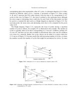
Figure 4.10. HCF limit strength with and without LCF pre-damage: (a) R
HCF
= 05, (b) R
HCF
= 01,
(c) R
HCF
=08.
LCF–HCF Interactions 157
Fatigue strength (MPa)
(c)
850.0
870.0
890.0
910.0
930.0
950.0
No. pre-damage 700
MPa, 0.1R
500,000 cycles
900

MPa, 0.5R
50,000 cycles
Figure 4.10. (Continued).
to be higher than the baseline. The observation that they were lower suggests that there
might be an effect of pre-damage due to LCF, but the magnitude is not significant.
In Figures 4.10b, c, results are shown where LCF was applied at a stress of 900 MPa on
a titanium alloy that has a yield stress of 930 MPa. In this case, strain ratcheting occurred
during the LCF portion of the test, but no ratcheting was observed in the HCF portion
of the test under step-loading conditions. Morrissey et al. [16] have reported that time-
dependent creep or ratcheting may play an important role at high stress ratios where a
portion of each cycle is spent at stresses near or above the static yield stress of the material.
They observed measurable strain accumulation dependent on the number of cycles, as
opposed to time, at the stress ratio of 0.8 where the applied maximum stress was slightly
above 900 MPa. The fracture surfaces for the cases where strain ratcheting was observed
in the tests summarized in Figure 4.10 did not show any indication of this phenomenon.
This is in contrast to the observations of Morrissey et al. [16] where ductile dimpling
was observed on fracture surfaces on specimens tested at R =08 with maximum stresses
above approximately 900 MPa. In fact, over the range of conditions studied in [14], there
appeared to be little or no effect of prior LCF on the subsequent HCF limit stress. If any
cracks formed during LCF, they were not observable through fractography and were not
of sufficient size to cause any significant reduction of HCF limit stress under subsequent
158 Effects of Damage on HCF Properties
testing. So, for conditions that covered a range from overloads to underloads from LCF,
there was no observable effect on the subsequent HCF limit stress in a titanium alloy.
A similar investigation into load-history effects on the HCF limit stress was conducted
by Morrissey et al. [15] where an attempt was made to assess the damage that might
occur from HCF transients when these transient stresses exceeded the undamaged HCF
limit stress. They addressed a practical problem that arises in designing against HCF
because of the possible occurrence of stress transients above the FLS. These stress levels
can correspond to lives below the HCF limit, but not necessarily to those which produce

LCF. The slope of the S–N curve is quite shallow in this region, making the scatter in
the cycles to failure quite large and, consequently, making cycle counting difficult from
a deterministic life prediction scheme.
As shown in the previous section, the effects of prior loading under LCF seem to have
little or no effect on the subsequent HCF limit stress, even when loading under LCF has
covered life ranges as high as 50–75% of anticipated life in both smooth and notched
specimens. To investigate effects due to transient loading, Morrissey et al. [15] used high
frequency blocks of loading to represent the cumulative effect of HCF transients which
might cause crack initiation to occur. They determined the effects of these transients for
two reasons. First, short duration, high frequency stresses above the fatigue limit (but still
within the HCF regime) are typical of what occurs in gas turbine engine applications.
Second, in contrast to LCF overloads that would by definition only occur for a very small
number of cycles, HCF stress transients could produce large numbers of cycles, even if
they only occur for up to 20% of the expected fatigue life at that stress.
The experiments in [15] involved the application of HCF transient stress levels for
a certain percentage of life (ranging from 7.5 to 25%) and then using the step-loading
technique to determine the subsequent fatigue strength corresponding to 10
7
cycles at
R =05. Some specimens were either heat tinted or both heat tinted and stress relieved
(SR) after the pre-cycling (prior to HCF testing). The results are summarized in Table 4.1
which presents the ratio of the final failure stress under HCF loading conditions, 
f
(after
applying stress transient loads) to the 10
7
cycle HCF endurance limit, 
e
. It is clear
from the table that preloading at 855 MPa (30% above the endurance limit) for 50,000

cycles (approximately 25% of life) does not reduce the subsequent HCF strength of the
Table 4.1. Summary of fatigue limit stress results for specimens subjected to stress transients
# of tests 
LCF
N
LCF
% of life 
f
/
e
3 855 50000 25 0.99
5 925 25000 25 0.92
3 925 15000 15 0.94
1 925 7500 75 0.93
3 925 (SR) 25000 25 0.81
LCF–HCF Interactions 159
material. Table 4.1 also shows that cycling at 925 MPa for up to 25% of life has little
effect on the HCF strength. However, the HCF strength is reduced by an average of
19% when subjected to prior cycles with a maximum stress of 925 MPa followed by a
stress relief process. This implies that there are residual stresses present after the stress
transient cycling that act to reduce any loss in HCF strength. The nature of these stresses
might be attributed to crack closure, residual compressive stresses ahead of the crack tip,
or other phenomena. The net effect is one similar to what is commonly seen in crack
growth studies under spectrum loading and is referred to as an overload effect, where
prior cracking at a high load level tends to retard crack extension at lower loads.
To analyze the experimental data, a Kitagawa diagram was constructed for a circular
bar, the geometry used in the experiments. The resulting diagram is shown in Figure 4.11
where the parameters are given in the figure and no correction is shown for short cracks.
The crack growth analysis for the curve is presented below. For comparison, the diagram
shows the line for a simple edge-crack geometry for a material having the same endurance

limit as well as long-crack threshold stress intensity. This simple example also illustrates
the dependence of the shape of the Kitagawa diagram on the specific geometry and value
of R being used.
The crack growth analysis in [15] was also made in order to distinguish the initiation
stage from the total life observed experimentally. The approach was to subtract the crack
propagation time from an initial crack size a
0
from the total life to failure, where a
0
is
the transition crack size in the Kitagawa diagram. When repeated over the range of stress
levels used for the coupon fatigue tests, the result is a stress-life curve for nucleation life
compared to the stress-life curve for total life.
100
1000
10
1
10
2
10
3
Circular bar
Edge crack
Endurance limit
Maximum stress (MPa)
Crack depth (μm)
Ti-6Al-4V plate
R
= 0.5
K

max,th
= 6.38 MPa

σ
e
= 660 MPa
a
0
= 29.7 μm
a

0
= 68.1 μm
200
400
600
800
Figure 4.11. Kitgawa diagram for a circular bar.
160 Effects of Damage on HCF Properties
The Forman and Shivakumar [17] stress intensity factor for a surface crack in a rod can
be used for this analysis. This solution assumes that cracks have a circular arc crack front
whose aspect ratio starts as 1.0 for small cracks. As the crack propagates, the aspect ratio
changes according to experimental observations that are embedded in the K solution.
Therefore, only the crack depth, a, is used in the solution. The crack depth is defined as
the radial distance from the circumference to the interior of the crack. Equation (4.11)
is the general form of the stress intensity factor solution. The geometry correction factor
F
0
, defined by Equations (4.12) and (4.13), is dependent only on the ratio of crack size

to rod diameter,  [Equation (4.14)].
K
I
=


0
F
0


√
a (4.11)
F
0
 =g

0752 +202 +037

1−sin 

2

3

(4.12)
g =092

2




tan 

2


2

1/2

sec

2

(4.13)
 =
a
D
(4.14)
To calculate the propagation life of the fatigue tests from an initial crack size, a crack
growth law must be defined. The crack growth rate da/dN versus the stress intensity
factor range K was based on experimental data for the same Ti-6Al-4V used in this
study [18].
da
dN
=465×10
−12
K
389

(4.15)
The propagation analysis procedure is, for each stress level, to start with the defined
initial crack size a
0
, calculate K, and then calculate the crack growth rate da/dN .
A small increment of crack growth, a, is then applied and the corresponding increment
of cycles, N , is calculated. This procedure is repeated until failure when K
max
equals
the fracture toughness K
c
that is approximately 60MPa
√
m for this material.
As discussed above, a Kitagawa type diagram can be useful in evaluating the potential
for a crack to reduce the HCF capability of a material. Since stress transients above the
HCF endurance limit were being introduced to the material, the possibility that cycling
at these stress levels resulted in cracking was evaluated numerically. For this purpose,
a Kitagawa type diagram was constructed for the experimental conditions under consid-
eration. The endurance stress, 
e
, was taken as the value that had been experimentally
determined and the crack growth threshold curve was developed using the K solution
above for a crack on the surface of a cylindrical bar. The resulting diagram is shown in
Figure 4.12, along with the El Haddad short crack correction. The crack length, a
0
, used
LCF–HCF Interactions 161
100
1000

11010
2
10
3
Kth,LC
Kth,SC
KOL,LC
KOL,SC
Stress (MPa)
Crack length, a (μm)
σ
e
0.81σ
e
0.93σ
e
a

0
Figure 4.12. Kitagawa diagram with model for overload and short crack corrections. Data points correspond
to fatigue limit stresses of LCF–HCF samples with and without stress relief. SRA samples should
follow non-model curve, non-SRA should have overload effect. Dots show what fatigue limit
stresses imply initial crack lengths might be. No such cracks were found.
for the El Haddad short crack correction was determined from the intersection of the
threshold curve with the endurance limit stress as a
0
=57m.
The crack sizes corresponding to the threshold for crack propagation at a given FLS,
due to an initial flaw which may have been produced during initial cycling, can be
represented on a Kitagawa diagram for the specific geometry used here, a circular bar.

For the specimens that were stress relieved to eliminate any prior load-history effects,
this diagram shows that, with the small crack correction and the experimentally observed
FLS of 081
e
, a crack of length approximately 30 m in length would produce that
threshold stress. On the other hand, specimens that saw no stress relief might exhibit an
overload effect due to the initial cycling which occurred at a maximum stress level above
the stress obtained during the HCF FLS tests. The magnitude of the overload effect on
the threshold for subsequent crack propagation was estimated from a simple overload
model developed in [6] that assumes the overload effect is caused by the prior loading
history and depends on K
max
of the prior loading. The model prediction for the history
dependent threshold is
K
maxth
=
K
eff
th

1−R
th

+


1−R
th


K
maxpc
(4.16)
where  = 0 294 and K
eff
th
= 323, are fitting parameters taken from [6]. Subscripts
“th” and “pc” refer to the threshold test and the precrack from the prior LCF loading,
respectively.
162 Effects of Damage on HCF Properties
The numerical results using the overload model for a stress of 925 MPa are plotted
in Figure 4.12 along with the small-crack correction corresponding to a value of a
0
=
92 m , as determined from the model and the endurance limit stress. This model should
correspond to the experimental observations where no stress relief was used, where
the fatigue limit for prior loading history at 925 MPa for a range of cycle counts was
approximately 093
e
(see Table 4.1). For this value of stress, the overload model shows
that a crack of approximately 20 m in length would be expected to produce the threshold
stresses obtained experimentally. In the case of no stress relief, or with stress relief as
indicated above, the initial cycling is expected to produce a crack of length 20–30 m
in order to explain the observed reduction in FLS. In both cases, the size of any crack
developed during LCF is near the limit of detection, using either SEM or heat tinting, but
more importantly, does not have any serious detrimental effect on the subsequent FLS.
In order to determine the expected flaw size that might occur due to prior cycling, the
crack growth life was calculated as noted above. The crack growth life for any value
of applied stress is subtracted from the total life to produce a curve corresponding to
an initiation life to a crack of length a

0
= 57m. The results are plotted in Figure 4.13
in terms of percent life spent in nucleation, where it can be seen that the initiation of
a crack to the size of a
0
should not be expected after the number of cycles imposed in
the experiments as shown in Table 4.1. For example, at the highest stress of 925 MPa,
the expected total life is approximately 10
5
cycles. At that stress, the percent of life
spent in nucleation to a crack length of a
0
is expected to be about 50%. Thus, initiation
corresponds to approximately 50,000 cycles, twice as much as the 25,000 imposed in
the experiments. From this it is concluded that fatigue cycling for fractions of life below
50% should not produce a detrimental effect on the subsequent HCF endurance limit.
0
20
40
60
80
100
N
f

(cycles)
Percent of life in nucleation
10
4
10

5
10
6
10
7
Figure 4.13. The percent life spent during nucleation as a function of the coupon fatigue test failure life.
LCF–HCF Interactions 163
Since the cyclic life is a statistical variable, a factor of 2 in life should be within expected
statistical scatter and the design life should be typically much less than the lives plotted
from a limited number of experiments that determine average values.
LCF–HCF interactions have also been studied by applying loading from other than
smooth bars subjected to uniform stress. One example is where C-shaped specimens were
precracked during fretting fatigue studies and were subsequently evaluated to determine
the threshold for fatigue crack propagation [19]. Data for cracks in C-shaped specimens
are plotted on a Kitagawa diagram as shown in Figure 4.14 for HCF limit stresses
obtained at R =01. A similar plot for data at R =05 is shown in Figure 4.15. The small
crack data for a<a
0
seem to be well represented by the El Haddad line and endurance
limit stress, while the longer crack data are well represented by the long crack threshold
fracture mechanics parameter, K = K
lc
th
. A large number of data points for small cracks
were obtained because, under fretting fatigue conditions, the contact stress field extends
only tens of microns into the contacting bodies. Thus, cracks can initiate at the surface
due to very high contact stresses there, but the cracks arrest quickly as they propagate
into the fretting pad from which the C-shaped specimens were cut. Fretting fatigue is
discussed in more detail in Chapter 6.
Some of the specimens were stress relieved (denoted by Stress relief annealing [SRA]

in the figures) to eliminate residual stresses and corresponding load-history effects from
the fretting fatigue testing. Each of the figures presents three lines, one is the long crack
solution, presented next, one is the short crack corrected solution (dashed line), and one
is the FLS for this particular C-shaped geometry obtained experimentally for each value
of R. The maximum threshold stress averaged 552 MPa for R = 01 and 684 MPa for
R =05.
100
200
300
400
500
600
700
1 10 100
Experiment
Experiment with SRA
Prediction w/o correction
Prediction with a
0
correction
Maximum stress (MPa)
Crack depth, a ( μm)
800
500
Fatigue limit
R = 0.1
ΔK
th

= 4.56 MPa√m

Figure 4.14. Kitagawa type diagram for HCF threshold stresses in C-specimens, R =01.
164 Effects of Damage on HCF Properties
100
200
300
400
500
600
700
1 10 100
Experiment
Experiment with SRA
Prediction w/o correction
Prediction with a
0
correction
Maximum stress (MPa)
Crack depth, a (μm)
800
500
Fatigue limit
R = 0.5
ΔK
th

= 3.46 MPa√m
Figure 4.15. Kitagawa type diagram for HCF threshold stresses in C-specimens, R =05.
The values of long crack K
th
used were 4.6 and 29MPa

√
m for R = 01 and 0.5
respectively. The R = 0.1 data followed the predictions quite well. The R = 05 data
were more scattered but also followed the same trend. A majority of the data fell into the
long crack region where LEFM clearly predicted the threshold. Some of the specimens,
however, had cracks on the order of a
0
and these data clearly deviated from LEFM and
followed the trend of the small crack threshold model. It is also apparent, by observing
the trend of the curves in Figures 4.14 and 4.15 that the small crack correction not only
represents the trend of the experimental data, but shows that for crack lengths much
below a
0
that the FLS is not appreciably below that of an uncracked body. Thus, if
assessing the potential damage of a fretting induced crack, the FLS of a body with a
“small crack,” below a
0
, is not much lower than that of an uncracked body even though
the calculated value of K may be much reduced from that in a long crack experiment.
For small cracks, therefore, stress rather than K should be considered as the governing
parameter when assessing potential material degradation from fretting fatigue. Overall,
the Kitagawa diagram, using the El Haddad transition modification, provides a reasonable
representation of all of the experimental data including those in the small crack regime.
A stress intensity factor K analysis of this specimen was required for the fatigue
crack growth threshold analysis. The fretting cracks in the C-specimens were modeled
as semi-elliptical surface cracks in a plate as drawn in Figure 4.16. The stress gradient
of the uncracked specimen was used to calculate K for the cracked specimen by the
well-known superposition method. Since this stress gradient was not linear, a generalized
weight-function solution was used as presented in Shen and Glinka [20]. Equations (4.17)
and (4.18) were used to evaluate K at the depth and surface points of the semi-elliptical

crack. In these equations, K
A
and K
B
are the mode I stress intensity factors at the depth
LCF–HCF Interactions 165
2W
t
a
2c
x
A
B
Figure 4.16. Surface crack in plate geometry used for K analysis in C-shaped specimens.
and surface points respectively, x is the stress gradient along the crack depth, and
m
A
and m
B
are the weight functions. The weight functions are defined in Equations
(4.19) and (4.20). The six coefficients, M
iA
and M
iB
, were derived with the use of known
K solutions for tension and bending. The coefficients depend on the crack size, crack
shape, and plate geometry.
K
A
=


a
0
x m
A

x a
a
c

dx (4.17)
K
B
=

a
0
x m
B

x a
a
c

dx (4.18)
m
A
x a =
2


2a −x

1+M
1A

1−
x
a

1/2
+M
2A

1−
x
a

+M
3A

1−
x
a

3/2

(4.19)
m
B
x a =

2

x

1+M
1B

x
a

1/2
+M
2B

x
a

+M
3B

x
a

3/2

(4.20)
In evaluating the results of this investigation, a result of particular interest is the fact
that for very small cracks, the stress levels at the threshold are those at or slightly below
the endurance limit stress for uncracked specimens. However, the location of failure is
found to be at the pre-existing crack as observed from fracture surfaces that were heat

tinted before threshold testing in order to provide the dimensions of the pre-existing
crack. A legitimate question could be raised about why failure did not occur at a location
other than the precrack since the applied stresses were approximately those corresponding
to the endurance limit stress. In other words, if very small cracks do not degrade the
stress carrying capability of the material, why do they provide the location for subsequent
failure? Note that we are dealing with a fatigue limit or threshold condition, not a number
of cycles to failure where number of cycles to initiation is an important part of the