High Cycle Fatigue: A Mechanics of Materials Perspective part 20 pot

176 Effects of Damage on HCF Properties
K
t
= 1.94
K

t
= 2.25
c
a
Fracture
surface
1.27
70
1.27
1.27R
2.03R
35
10.16
1.27
All dimensions
in mm
Figure 4.21. Double-notch-tension specimen geometry and crack shape nomenclature.
Time
K
K
th
max
K
th
min

K
r
ΔK
th
eff
Precrack Threshold test
K
pc
max
Figure 4.22. Schematic of LCF–HCF loading history and nomenclature.
LCF–HCF Interactions 177
100
200
300
400
10 100
20 50 200
R
LCF
= 0.1, σ
max

= 430 MPa
R
LCF
= –1.0, σ
max

= 265 MPa
K

max
= 5.1 MPa√m, R = 0.1 a/c = Fit
R
= 0.1 Fatigue limit stress (10
7
cycles)
σ
max
(MPa)
c (μm)
R
HCF
= 0.1
Figure 4.23. HCF thresholds at R =01 on a Kitagawa type diagram.
100
200
300
400
10 100
σ
max
(MPa)
c (μm)
R
HCF
= 0.5
20 50 200
R
LCF
= 0.1, σ

max
= 430 MPa
R
LCF
= –1.0, σ
max
= 265 MPa
K
max
= 5.8 MPa√m, R = 0.5 a/c = Fit
R
= 0.5 Fatigue limit stress (10
7
cycles)
Figure 4.24. HCF thresholds at R =05 on a Kitagawa type diagram.
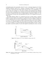
The horizontal line in each figure represents the experimentally determined endurance
limit of the uncracked specimen corresponding to 10
7
cycles. It can be seen in both
figures that the data obtained using LCF at R = 01 (circles) show what appears to be
equivalent to an overload effect since the threshold values of stress are consistently above
the extrapolated long crack threshold. Conversely, data obtained using LCF at R =−10
(triangles) tend to fall slightly below the projected long crack threshold, the type of effect
being representative of what one would expect when a material sees an underload during
prior cycling. These results seemed to indicate that an overload type condition (LCF at
R =01) retards the subsequent HCF propagation while an underload (LCF at R =−10)
might tend to slightly accelerate the subsequent HCF propagation. The apparent overload
effect from precracking at a higher stress than that required to propagate the crack
178 Effects of Damage on HCF Properties
under HCF is the result of multiple “overloads” since constant amplitude loading was

used to precrack the specimens. The apparent multiple overload effect is consistent with
observations such as those of Frost [41] who noted that cracks formed by precracking
at a higher alternating stress are all stronger than expected and that the “propagation
stress” (stress to obtain K
th
) is increased if the initial loading conditions are such as to
induce compressive residual stresses at the crack tip. It should also be noted here that the
overload ratios (OLR = ratio of precrack stress to FLS) in the works of Moshier et al.
were relatively small compared to those used in typical studies of overload effects where
values of OLR commonly exceed 1.5 in order to produce noticeable effects [42]. While
it is not the intent of this book to discuss the governing mechanisms of retardation due
to overloads, the reader is referred to the review article by Sadananda et al. [42] who
address that subject.
In the Kitagawa diagram used to present the threshold data above, all combinations of
crack length and stress corresponding to a K solution equal to the threshold value can
be plotted to establish the threshold crack-growth line. Although small crack corrections
were not used here, the concept of data points below the endurance limit represents a
threshold for cracks of a particular size. It is clear that such cracks could not be naturally
initiated since they represent stress levels below the endurance limit. While such cracks
could be preexisting in the material in the form of initial defects, material with such
defects in sufficient quantities would have a lower endurance limit (by definition!). It
follows, therefore, that data plotted on a Kitagawa diagram representing a crack length
and stress below the endurance limit generally represent a condition where the crack was
initiated above the endurance limit. The question can be raised as to whether any point
on a Kitagawa diagram is unique or, instead, is dependent on the history of loading in
getting to that point. The long-crack threshold, for example, represents a data point that
may be dependent on loading history. While standards have been set for determining this
threshold by following a predetermined loading history, the history dependence and the
existence of a unique long-crack threshold still have to be questioned. This subject is
discussed further in Chapter 8.

Noting that prior loading history involving multiple overloads and underloads can influ-
ence measured FCG thresholds in surface cracks at notches, Moshier et al. [6] conducted
a series of long crack experiments to further study the load-history effect on threshold.
The study was conducted on both Ti-6Al-4V (Ti-6-4) and Ti-5Al-2Sn-2Zr-4Mo-4Cr (Ti-
17). They measured the threshold under constant R, HCF loading, using an increasing
K step-loading procedure as shown above (Figure 4.22). LCF precracking was done
using a range of K values where the corresponding K
max
representing LCF loading was
greater than those of the subsequently measured HCF thresholds, thereby producing the
multiple overload condition. This condition is represented schematically in Figure 4.22.
Data obtained at R
HCF
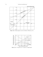
=0.1 showed a linear relation between the HCF threshold and the
K
max
and R values of the LCF precrack for long cracks in C(T) specimens. Figures 4.25
LCF–HCF Interactions 179
0
2
4
6
8
10
12
0 5 10 15 20 25
R = 0.1
R = 0.1 SRA
ΔK
th

(MPa√m)
ΔK
Precrack
(MPa √m)
ΔK
th
= 0.303 ΔK
Precrack
+ 2.999
4.6 MPa √m
Load shed threshold
Figure 4.25. Threshold data at R = 01 for Ti-6Al-4V with and without stress relief annealing (SRA)
R
LCF
= 01.
and 4.26 show the observed linear relationship between K of the (LCF) precrack and
the K threshold for testing at R
HCF
= 0.1 for Ti-6-4 and Ti-17, respectively. A similar
plot to Figure 4.25 that includes small-crack specimen data is presented in Figure 4.27
and shows that small-crack data follow the same linear trend. A number of the precracked
specimens were SRA to remove any residual stresses developed in the precracking. It
can be observed that for SRA, the threshold obtained is independent of precrack history
in both materials. The data also agree fairly well with the long-crack threshold obtained
under conventional load shed techniques, shown in the figures as “Load Shed Threshold.”
However, the data from SRA lie slightly below the long crack threshold, more for Ti-6-4
than for Ti-17. The authors speculated that the reason for the slightly lower threshold
is that SRA completely eliminates load-history effects and residual stresses whereas the
0
2

4
6
8
10
12
0 5 10 15 20 25
R = 0.1
R
= 0.1 SRA
ΔK
th
(MPa√m)
ΔK
Precrack
(MPa√m)
ΔK
th
= 0.366 ΔK
Precrack
+ 2.137
3.5 MPa√m
Load shed threshold
Figure 4.26. Threshold data at R =01 for Ti-17 with and without stress relief annealing (SRA) R
LCF
=01.
180 Effects of Damage on HCF Properties
0
2
4
6

8
10
12
0 5 10 15 20 25
Long crack R = 0.1
Long crack R = 0.1 SRA
Small crack R = 0.1 LCF
ΔK threshold (MPa √m)
ΔK
Precrack
(MPa √m)
R = 0.1 HCF
ΔK = 4.6 MPa√m
Long crack threshold
Figure 4.27. Experimental relationship between precrack and threshold stress intensity for R = 01 threshold
tests in long crack C(T) specimens and small surface flaws.
long crack threshold retains whatever residual stresses or closure is present at the end of
the conventional load-shed procedure for threshold testing. The resulting threshold could
even be considered to be a “true” material threshold, although no such definition of a
true threshold seems to exist.
To represent the linear relation between K
th
of the HCF testing and the K
Precrack
,a
simple model was developed to fit the data and to use in follow-on analytical modeling
of other load-history-dependent threshold test results. The model is purely empirical in
nature and was not intended to be a general overload model, many of which already exist
in the literature.
4.3.1.1. An overload model

While overload models to estimate FCG retardation abound in the literature, there are
few to estimate thresholds. A model for estimating threshold from the LCF precrack level
was developed using an approach similar to those used in closure and crack retardation
modeling. From the data shown in Figures 4.25 and 4.26 for long cracks in C(T) specimens
in both Ti-6-4 and Ti-17, an effective threshold was found to be a material constant. This
was used to formulate a relationship between K
max
threshold and K
r
, where K
r
is defined
as the stress intensity factor level above which K is effective and below which it is not.
This reduces the stress intensity factor range to an effective range:
K
eff
th
=K
max
th
−K
r
(4.21)
where the various terms are defined in the loading schematic, Figure 4.22. K
r
is analogous
to the opening stress intensity factor K
op
used in closure-based models, and K
pr

, the crack
LCF–HCF Interactions 181
propagation intensity factor [42]. After many iterations to consolidate the experimental
data, K
r
was found to be best represented in the form
K
r
=

K
max
pc
+K
min
th

(4.22)
where  is a fitting parameter and subscripts “pc” and “th” refer to the LCF precrack and
HCF threshold, respectively. The effective stress intensity factor range, K
eff
th
, is assumed
to be a material constant representing the minimum effective K to propagate a crack.
The linear relation between K
th
and K
pc
, observed experimentally, is then written as
K

th
=

1−R
th

K
eff
th

1−R
th

+


1−R
th


1−R
th


1−R
pc

K
pc
(4.23)

The linear fit of threshold data at R = 01 was used to determine the parameters K
eff
th
and  K
eff
th
= 323 and  = 0294 for Ti-6-4 and K
eff
th
= 229 and  = 0353 for
Ti-17). This model was then applied to data obtained at different values of R for the
HCF threshold testing. The ability of this equation to represent threshold data obtained
at these other values of R after precracking at R = 01 is illustrated in Figure 4.28 for
long cracks in C(T) specimens for Ti-6-4. The empirical fit to the data is made only for
the data obtained at R = 01. The fit at R =01 provides the constants which, in turn,
produce the model predictions shown for other values of R in the figure. It can be seen
that the model provides an excellent representation of the entire data set. An equally
good correlation was obtained for T-17 by fitting the data at R =01 and predicting the
behavior at R =05 and R =07 (see [6], Figure 4.5).
0
2
4
6
8
10
12
0 5 10 15 20 25
R

=

0.1 Expt
R

=

0.3 Expt
R

=

0.5 Expt
R

=

0.7 Expt
R

=

0.3 Model
R

=

0.5 Model
R

=

0.7 Model
R

=

0.1 precrack
Δ
K
Precrack
(MPa√m)
Δ
K
threshold (MPa√m)
Figure 4.28. Experimental data and model predictions for long crack data.
182 Effects of Damage on HCF Properties
4.3.1.2. Analysis using an overload model
For the general case of an overload model applied to any geometry, the K solution for
the specific geometry is written in the form
K = 
√
a fa (4.24)
Denoting the precrack condition with subscript pc, the K used to produce an overload
condition, which we refer to as the LCF precrack, is
K
pc
=
pc
√
a fa (4.25)

For the particular overload model used here, the linear relation between K
th
and K
pc
,
Equation (4.23), requires K
th
= K
pc
when there is no overload as in the limiting case of
steady-state crack growth near threshold. In this case, K is the long crack threshold, K
lc
th
,
a material constant, and Equation (4.23) can be rewritten as
K
th
=K
pc
+K
lc
th
1− (4.26)
where  is an empirical constant. In these equations, K represents the maximum value
of K at a given value of R, but could also represent K throughout.
To extend the modeling to small cracks, the concept of El Haddad et al. [3] is employed
to produce the endurance limit stress for arbitrarily small cracks, and the K solution,
Equation (4.24) for long cracks. Following the procedure of modifying the material
capability (threshold stress intensity) instead of the crack length, the threshold value of
K, denoted by

K
th
, is reduced for small cracks in the following manner:
K
th
=K
th

a
a +a
0

1/2
fa
fa+a
0

(4.27)
where a
0
, as defined by El Haddad, and modified for the more general K solution of
Equation (4.24), is given by Equation (4.4) previously, but repeated here:
a
0
=
1


K
th


e
fa
0


2
(4.28)
which can be solved for a
0
either graphically or iteratively. The crack length a
0
is usually
not considered in the fa term of Equation (4.24) when deriving the effective K in
Equation (4.27). For each crack length, the threshold stress is obtained from a combination
of Equation (4.27) and the K solution, Equation (4.24), in the following equation:
 =
K
th
√
a fa
(4.29)
LCF–HCF Interactions 183
4.3.2. Examples of LCF–HCF interactions
As an illustrative example, a SEN specimen is cracked at a stress corresponding to the
endurance limit, 
e
, and another one at a stress above the endurance limit,  =125
e
in

this case. The K solution is approximated in Equation (4.24) by setting fa = 1. From
the K solution, and the small-crack correction, Equation (4.27), the threshold condition
for a baseline chosen arbitrarily as K
th
= 5 MPa
√
m and 
e
= 300 MPa is represented
in the form of a Kitagawa type diagram in Figure 4.29. The diagram shows the smooth
transition from a fracture mechanics dominated long-crack threshold, where the slope on
a log-log plot is −05, Equation (4.24), to a crack-length independent endurance limit,

e
= 300 MPa, for arbitrarily short cracks. If, however, the crack is initiated at a stress
equal to or above the endurance limit,  =
e
and  =125
e
for the two cases here, then
the longer the crack developed under this “LCF” or precrack condition, the higher will
be the value of K
OL
as determined from Equation (4.25). For each case modeled, pairs
of values of a and K
pc
are obtained. Then K
th
can be calculated from Equation (4.26)
and modified for short cracks using Equation (4.27) to get an effective value of K

th
. The
relation between  and a is obtained from Equation (4.29) to determine points on the
Kitagawa diagram as illustrated in Figure 4.29. The divergence of the curves for  = 
e
and  = 125
e
is due to a combination of the increase in K
pc
due to increase in LCF
crack length, as well as the form of the specific model used here, Equation (4.26), which
shows that the threshold increases with increase in K
pc
. The assumption implied in this
illustrative analysis, which could be applied to any actual experimental geometry, is that
the endurance limit is a material constant at a given R and does not depend on any prior
load history which does not produce cracks. This assumption has been validated under
several experimental conditions described at the beginning of this chapter. The net result,
20
40
60
80
100
300
10
–1
10
0
10
1

10
2
10
3
10
4
Overload model
σ
e
=

300 MPa
K
th
=

5 MPa√m
Baseline
σ = σ
e
σ = 1.25σ
e
Stress (MPa)
Crack length (μm)
Figure 4.29. Kitagawa diagram for theoretical SEN specimen behavior.
184 Effects of Damage on HCF Properties
as shown in Figure 4.29, is that the stress required to produce growth of a crack under
HCF, which developed under constant load at or above the endurance limit, is below the
endurance limit stress but above the baseline stress calculated from fracture mechanics
with a small crack correction. The difference is attributed to the load-history effect.

The concept and model described above was applied to an expanded database from
experiments on notched specimens in which very small cracks could be detected [4]. The
K solution was obtained for the notch geometry with a surface flaw, and the overload
effect on the threshold for K was obtained from the model, Equation (4.23). To account
for a small crack effect, K was then modified in accordance with Equation (4.27). The
specific value of the a/c ratio in the K solution was used for each data point in the
calculation of a
0
which is where the endurance limit stress and K
th
equation cross on
a Kitagawa diagram. The data and the model fit are shown in a Kitagawa diagram in
Figure 4.30 where the model prediction is based on Equation (4.23) with the appropriate
fit to data from long crack experiments.
The data, summarized in Figure 4.30, include tests where both R =−1 and R = 01
were used for the LCF precracking and both SRA and no stress relief were applied prior
to HCF testing for both cases. LCF precracking produced cracks with depths covering a
range from c =16 to 370m. For modeling predictions, three curves are shown. In one
case, the threshold from long cracks (K
max
=51 MPa
√
m) is used without any overload or
small crack correction. This corresponds to Equation (4.24) with K being a constant using
the appropriate aspect ratio in the K solution. The second analytical curve corresponds
to a prediction without any small crack correction. This simply incorporates the overload
effect, Equation (4.23), in the calculation of K
th
. The third prediction is identical, but
the small crack effect is taken into account through the use of Equation (4.27). Several

100
200
300
1 10 100
LCF R = 0.1
LCF R = –1.0
LCF R = 0.1 with SRA
LCF R = –1.0 with SRA
Long crack ΔK
th
Long crack ΔK
th
with a
0
Prediction without a
0
Prediction with a
0
Maximum stress (MPa)
Crack depth, c (μm)
400
500
Fatigue limit
Figure 4.30. Experimental data and model predictions on a Kitagawa diagram.
LCF–HCF Interactions 185
features of the analytical predictions should be noted. First, the curve for constant K is
not a straight line of slope −05 as is often noted in a Kitagawa diagram. The reason
for this is that the K solution is of a more complex form, Equation (4.24), than for the
simple case where fa =1 corresponding to the simple
√

a dependence of K on crack
length. The second feature for the cases of a constant load to produce an overload effect is
that the model predicts behavior quite different than the constant K solution as illustrated
for the simple illustrative example shown in Figure 4.29.
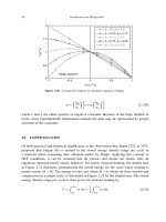
The correlation of the data with the analytical models, as shown in Figure 4.30, shows
the ability to extend a long-crack overload model to small surface flaws in a notch
geometry. The cracks developed under R =01 loading have thresholds at R =01 which
are predicted, somewhat conservatively, by the linear overload model of Equation (4.23)
with the small crack (a
0
) correction of El Haddad. It is clear from the data that the
threshold is increased when there is an overload history applied during the LCF stage,
similar in concept to the retardation effect observed in growing cracks. LCF cracks formed
under R =−1 loading, on the other hand, produce thresholds which are predicted by the
(constant) long-crack threshold value of K
max
=51MPa
√
m. The maximum stress or K
level in the threshold testing exceeded that of the LCF precracking only for the smallest
crack formed in tests at R =−1 where precracking was at a maximum stress of 265 MPa.
The remainder at R =−1 and all at R =01 had lower values of K
max
in threshold tests at
R =01 than those in precracking. Thus all tests with the exception of one data point could
be expected to demonstrate some type of overload effect. However, unlike precracking
at R = 01, precracking at R =−1 seemed to have no overload effect on the subsequent
threshold. The compression portion of the fully reversed loading cycle appears to negate
any beneficial effect of the tension portion of the cycle upon the subsequent threshold.
For both prior loading at R =01 and R =−1, stress relief annealing produced a condition

where the subsequent threshold corresponded to the long crack threshold as shown by the
solid symbols in Figure 4.30. These data, as well as the data from precracking at R =−1
without SRA, show no history-of-loading effect on the subsequent threshold determined
at R = 01. The best representation of these threshold values would be the long crack
threshold with a small crack correction for the smallest of cracks in these tests. The small
crack correction can be seen in Figure 4.30.
Another important observation from the experimental data of Figure 4.30 is that for
cracks having depths, c, less than 30–40 m (the approximate value of a
0
as determined
by the intersection of the long crack threshold curve with the constant endurance limit
stress) is the value of the stress to produce crack extension. For these small cracks, while
calculated values of K might be considerably below the long crack threshold, the values
of stress at threshold are only slightly below or at the endurance limit stress within a
reasonable scatter band. This indicates that very small cracks are not very detrimental in
reducing the fatigue threshold stress, even though the location of the failure corresponds
to the location of the initial cracks.