High Cycle Fatigue: A Mechanics of Materials Perspective part 22 potx

196 Effects of Damage on HCF Properties
4.4.1. LCF–HCF nomenclature
Combined LCF–HCF loading has caused some confusion over the years because of
nomenclature and the differences that occur when dealing with actual usage versus
mathematical formulations involving simple linear summation concepts. Consider the
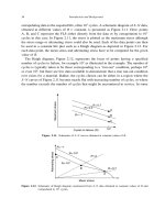
schematic of Figure 4.39 that shows the major cycles (LCF) with a hold or dwell time
in between them during which HCF cycles can occur. The problem we deal with is the
superposition of the HCF cycles on the LCF behavior. The nomenclature is that of Powell
and coworkers at University of Portsmouth, formerly Portsmouth Polytechnic.
LCF loading alone produces a stress intensity level K
major
and represents the contribu-
tion of the major throttle excursions in an engine. During dwell times, at maximum K for
the LCF cycle, a vibratory loading occurs whose total amplitude is denoted by K
minor
.
If the total contribution of the individual loading components is considered, then a linear
summation law would require that the total growth rate be the sum of K
total
+K
minor
,
not K
major
+K
minor
. This is because in the combined case, the effective amplitude of
the LCF cycles is K
total
, not K
major

, since the LCF cycle now goes from minimum to
maximum through an amplitude K
total
. This concept, while fairly clear, has not been
followed consistently in the literature over the years and has led to some confusion when
evaluating the applicability of a linear summation concept for crack growth under com-
bined LCF–HCF loading. The confusion arises because the minor cycle amplitude also
contributes to the major cycle amplitude as shown in the schematic of Figure 4.39.
Another point to consider in discussing combined LCF–HCF, referred to here as CCF,
is the manner in which the data are both recorded and discussed. While the stress or
load ratio, R, is a common and well-understood quantity, there are other parameters with
which to describe the entire load sequence in CCF, not including spectrum loading where
overloads, underloads, and sequencing also have to be considered. For the load ratios
we can use R
minor
and R
major
to represent the value of R for the HCF and LCF cycles,
respectively. The number of HCF cycles per LCF cycle is usually given by n. Unless the
value of n is sufficiently high, the contribution of the HCF cycles may not be detected
since the HCF is generally applied at a much smaller value of K than are the LCF
ΔK
major
ΔK
total
ΔK
minor
Figure 4.39. Schematic of combined major/minor cycle loading.
LCF–HCF Interactions 197
cycles. A parameter that is often used to represent the relative magnitude of the combined

stress cycles is the amplitude ratio, Q Q is defined as the ratio of the amplitude of the
minor cycles to the magnitude of the major cycles. It can also be written in terms of the
K values.
Q =
K
minor
K
major
(4.36)
Note again that the major cycle amplitude refers to K
major
as shown in Figure 4.39, not
to the value of K
total
even though the latter is used in linear damage summation. There
is no single, yet simple, way of relating the major and minor cycle ratios, other than
through the definition of Equation (4.36). The following useful expressions are easily
derived and are found frequently in the literature, particularly in the papers coming from
University of Portsmouth.
R
minor
=
2 −Q

1−R
major

2 +Q

1−R

major

(4.37)
Q =
2

1−R
minor


1−R
major


1+R
minor

(4.38)
In the example cited above, Figures 4.36 and 4.37, Q = 012 for R
major
= 01 and
R
minor
= 09. For parallel experiments with the same major cycle, higher amplitude
vibratory loading corresponds to Q =022 and R
minor
=082.
The crack-growth rate data from CCF are normally presented with respect to the
entire cycle block. Thus, as illustrated in Figures 4.36 and 4.37, the growth rate is
shown as da/dBlock where the block consists of a single LCF cycle with n HCF cycles

superimposed. For the horizontal axis, K
total
or K
max
can be used to describe the block
loading. As an alternative, K
major
can be used. In the latter case, the HCF data cannot be
shown superimposed on the block loading. A similar comment can be made for the use of
K
total
. If it is desired to represent the LCF, HCF, and CCF data on the same plot, the use
of K
max
is preferable. However, if a linear superposition concept is attempted graphically,
both a vertical shift to account for n HCF cycles per LCF cycle, and a horizontal shift to
account for the different maximum values in HCF and LCF has to be used. The reader is
cautioned that there is no easy way to show LCF, HCF, and CCF data on the same (log)
plot while also demonstrating linear summation graphically.
4.4.2. Example of anomalous behavior
An illustration of the type B behavior of Figure 4.35 observed in combined LCF–HCF
testing is taken from [52] where the fracture mechanics of a nickel-based single crystal
alloy was studied. The focus was on the interaction of HCF at high stress ratio and at
198 Effects of Damage on HCF Properties
high frequency combined with LCF at low stress ratio and low frequency in combined
cycle loading. The test plan utilized previous threshold data generated at 1100

F, for
R =01 and 0.8 in the <001/010> orientation on alloy PWA 1484. After precracking,
the specimen was run at a stress ratio of 0.1 at a frequency of 10 CPM (0.167 Hz) until a

crack length of a
i
was achieved. The target for a
i
was selected to be well below the K
max
threshold value for the R = 08 test data. A block of 1000 cycles of R = 08at60Hz
was then performed between each R =01 LCF cycle. This block loading was continued
until the calculated value for threshold at R = 08 was superseded at crack length a
f
.
After growing beyond the calculated value of the R = 08 threshold, the loading was
returned to LFC loading only at R =01. The test scheme was designed so that all loading
blocks could be performed on a single sample so that specimen-to-specimen variation
differences would not be included in the results. A schematic of the test approach is
shown in Figure 4.40.
For reference purposes, some specimens were tested under constant load to allow stress
intensity K to increase with increasing crack length to detect the onset of crack-growth
rate behavior of the R =08 cycles. The results of the first test under combined LCF–HCF
loading are presented in Figure 4.40 which shows that a sharp increase in crack-growth
rate occurred at crack length a
i
corresponding to the change in waveform from LCF to
LCF + HCF indicating that the R =08 (HCF) cycles did affect the LCF crack-growth rate.
This was in direct contradiction to the anticipated response based on the earlier R =08
threshold result that indicated the testing was below the HCF threshold. A return to pure
LCF loading resulted in the anticipated return to the original R = 01 trend. A second
specimen was then run to confirm that the data was repeatable and the same result was
achieved. The results of the second test sequence are shown in Figure 4.41. The open
circles indicate the HCF only test results showing the threshold region for HCF. As in

da /dN
LCF
a

o
a
f
a
i
LCF only
LCF + HCF
LCF only
σ
max
σ
max
0.1
0.1
0.8
0.1
σ
max
σ
max
σ
max
σ
max
σ
max

K

max
(ksi√in.)
Figure 4.40. HCF–LCF testing approach and prediction.
LCF–HCF Interactions 199
10
–8
10
–7
10
–6
10
–5
10
–4
10
–3
6 8 10 20
LCF only
LCF only
HCF only
HCF + LCF
LCF only
da

/dN

LCF
(in./cycle)

30
R
= 0.1 Threshold
97
K
max
(ksi in.)
Figure 4.41. LCF–HCF Interaction test results
the first test, the interaction between HCF and LCF produces an accelerated growth rate
below the HCF threshold.
To further study this unexpected crack-growth rate acceleration, five loading schemes
were devised and performed at a constant K
LCF
of 10ksi
√
in. The frequency was 10
cycles per minute (CPM) for the LCF portion and 60 Hz for the HCF portion. The loading
schemes are shown in Figure 4.42 as Case (a) through Case (f). A single sample was
again used to perform all six cases in succession with each case consuming up to 0.020 in
(0.5 mm) of specimen ligament before proceeding to the next case.
The results of the test sequence shown in Figure 4.42 are summarized in Figure 4.43.
Comparison of the various case loading blocks suggests the higher mean stress or dwell
is the significant contributor to the accelerated crack-growth behavior as opposed to the
number of HCF cycles. As shown in Figure 4.43, the application of dwell, Case (b),
increased the growth rate from the baseline without dwell, Case (a). The dwell produced
nearly the same acceleration as adding 1000R = 08 cycles, Case (c). The similarity
between Case (c) and Case (d) (1000 versus 500 HCF cycles) suggests that the sensitivity
to time-dependent behavior is inclusive of very small differences in hold times and
200 Effects of Damage on HCF Properties
= 0

N

HCF
N
LCF
16.7 s
Dwell
1000 500 1000 500
Case (a) (b) (c) (d) (e) (f)
σ
max
σ
max
σ
max
0.8σ
max
0.8σ
max
0.64σ
max
0.1σ
max
0.1σ
max
0.1σ
max
Figure 4.42. Constant K testing to identify crack-growth rate acceleration drivers.
10
–7

10
–6
10
–5
10
–4
0.1 0.12 0.14 0.16 0.18 0.2 0.22 0.24
(a)
(b)
(c)
(d)
(e)
(f)
da /dN (in./cycle)
Crack length (in.)
Figure 4.43. Test plan 2 results. Legend refers to loading blocks shown in Figure 4.42.
or cyclic frequency. In fact, threshold testing done previously on that program clearly
showed a pronounced frequency effect between 20 Hz, 1 Hz and 10 CPM (0.167 Hz).
An interesting aspect of these findings is that the results indicate that there is a dwell
effect present in a temperature regime well below what has typically been called the creep
regime. The significance of this finding is that very small decreases in frequency that is
10 CPM alone versus 10 CPM with as little as an 8-second dwell at maximum load, cause
up to a 2X–3X acceleration in crack-growth rate. One possible explanation proposed for
the LCF–HCF interaction effects was oxidation at the crack tip. Tests in vacuum were
recommended.
4.4.3. Another example of anomalous behavior
Another observation of the interaction of LCF and HCF and the subsequent growth rate
behavior is that of Russ [45] who conducted studies on Ti-17, a  processed titanium
alloy. In that work, LCF cycles with R =01 were superimposed on what are referred to
LCF–HCF Interactions 201

as “baseline” HCF cycles having R =07. Both cycles have the same value of maximum
load (or stress) for a given crack length. Data were obtained by decreasing the load to
obtain a pure HCF threshold and then increasing the load with the LCF–HCF spectrum
shown schematically in Figure 4.44. While the study uses the nomenclature of the HCF
cycles being the baseline, and the LCF cycles being the equivalent of an underload
(also called a negative overload in the literature), the phenomenology is identical to
that observed in the works described above (see [32–35] and Figure 4.39, for example).
In the work of Russ, the number of HCF cycles per LCF cycle was varied between
10 and 1000. Figures 4.45 and 4.46 show the observed growth rate behavior in the
region near the HCF threshold for HCF cycle counts of 200 and 1000 per LCF cycle,
respectively. Both figures show the trend expected if no interaction occurs, that is, if
linear summation of LCF and HCF growth rates is assumed. The experimental data appear
to demonstrate an accelerated growth rate under the combined loading as well as growth
rate acceleration below the expected HCF threshold. Although the value of R =07 for
the HCF cycles is high enough to expect the complete absence of closure, the author finds
that a combination of closure during the application of the R = 01 cycle and residual
deformation ahead of the crack may account for the interaction effect. From plane strain
finite element modeling, the author shows that closure develops immediately behind the
Time
K
Step down block
R
= 0.7, 500,000 cycles
Step up block
R
= 0.7, 500,000 cycles
R
= 0.1, 50 cycles
Figure 4.44. Schematic of load history for determining threshold for crack propagation under combined
LCF–HCF loading.

202 Effects of Damage on HCF Properties
10
–6
10
–5
10
–4
10
–3
10
–2
68910
P
max

=

1.77

kN
P
max

=

0.86

kN
Linear summation
da

/dB (mm/block)
157
K
max
(MPa m)
Figure 4.45. Fatigue-crack-growth rate results for 200 HCF cycles per LCF cycle.
10
–6
10
–5
10
–4
10
–3
10
–2
6810
P
max
= 2.85 kN
Linear summation
da

/dB (mm/block)
1579
K
max
(MPa m)
Figure 4.46. Fatigue-crack-growth rate results for 1000 HCF cycles per LCF cycle.

LCF–HCF Interactions 203
crack and compressive residual stresses develop ahead of the crack tip after the R =01
underloads. It should be pointed out that, consistent with FEM results by Sehitoglu et al.
[53], compressive residual stresses were observed even in the absence of closure during
the R =07 cycles. The distances over which the closure and residual stresses develop are
only a few microns, inviting speculation as to whether such phenomenology could affect
the net growth rate behavior. However, as in the previous examples of Type B behavior
as defined in Figure 4.35, the observed behavior is non-conservative when compared to
the predictions of a linear summation model.
Another observation by Russ [45] was on the threshold for crack propagation and the
differences in the growth rate behavior in the near-threshold regime. For a constant value
of K
max
= 8 MPa
√
m, Figure 4.47 shows the combined-cycle growth rate for different
numbers of HCF cycles per block (1 LCF cycle) as well as the results from a simple linear
summation of the individual contributions of LCF and HCF. For the maximum number
of HCF cycles per block, 1000, the growth rate is dominated by the HCF cycles. For
all conditions other than 10 HCF cycles per block, the experimentally measured growth
rates are higher than those predicted by the linear summation model. These differences
are approximately a factor of two or more. Equally important from a life prediction
point of view, the threshold for combined cycle loading is lower than predicted by linear
summation. For the spectrum illustrated in Figure 4.44, where the ratio of HCF to LCF
cycles is 10,000, the threshold value of K
max
for pure HCF is 727 MPa
√
m whereas,
during increasing loading for the combined cycle, the threshold at which crack growth

first appears is 699 MPa
√
m. While these differences in growth rate and threshold do not
appear to be very significant, Russ points out that the differences in fatigue lifetimes can
be significant when the combined cycling is in the region of the HCF threshold where a
significant portion of the total time for crack growth to failure takes place.
10
–6
10
–5
10
–4
10
–3
10
1
10
2
10
3
Experiment
Linear summation
da /dB (mm/block)
HCF cycles per block
K
max
= 8 MPa m
R
HCF
= 0.7

R
LCF
= 0.1
Figure 4.47. Fatigue-crack-growth rates for LCF–HCF spectrum of Russ [45].
204 Effects of Damage on HCF Properties
4.5. COMBINED CYCLE FATIGUE CASE STUDIES
There are other examples of combined cycle loading where HCF at stress levels below
their constant amplitude threshold appear to contribute to the combined cycle growth
rate. An example is the study by Zhou and Zwerneman [54] where the cycle block
contains small amplitude cycles with periodic overloads. Denoting the major cycles as
“overload” (ol) cycles and the other as minor cycles, the ratio K
minor
/K
ol
was chosen
as 0.3 and R
ol
= 01. A schematic of the block loading is shown in Figure 4.48. Using
ASTM A588 steel as the test material, values of the number of minor cycles per block,
n, were chosen as 0, 4, 9, 49, 99, and 999. The results, presented in terms of growth
rate per block, are shown in Figure 4.49. The number of cycles per block includes one
Time
K
n cycles
Minor
cycles
R
= 0.27
Overload
cycle

R
= 0.1
Figure 4.48. Schematic of block loading with periodic overload cycles.
10
–7
10
–6
10
–5
10
–4
1 10 100 1000
da /dBlock (in./cycle)
Cycles per block
Conventional
baseline
ASTM baseline
Figure 4.49. Fatigue-crack-growth rate for cycles with periodic overloads.
LCF–HCF Interactions 205
major cycle and n minor cycles. Since there is only one overload (major) cycle per block,
the increase in growth rate per block with increasing values of n can only be attributed
to the minor cycles. Yet the minor cycles are applied at K levels that are below their
constant amplitude threshold. The “conventional baseline” shown in the figure indicates
that there is no contribution due to the minor cycles. The assumed threshold for the minor
cycles was taken from an empirical formula for this material. If, instead, the ASTM
recommended value for threshold is taken as a growth rate equal to 10
−10
m/cycle, then
this small, but non-zero, contribution to the minor cycle growth results in the curve
labeled “ASTM baseline” in the plot. Even under this assumption, the data show that the

experimentally observed block growth rate is higher than predicted by a linear summation
rule. It is clear that the threshold is reduced by the overload cycles, an effect similar
to the acceleration of crack growth due to underload cycles observed by Russ [45],
described above. Further evidence of the growth due to the minor cycles was obtained
from acoustic emission (EM) monitoring. The intensity of the AE signals was observed
to increase with increasing numbers of minor cycles per block. The authors concluded
that the increase in AE activity indicated that “the minor cycles below the threshold
contribute to fatigue damage.” It certainly is possible that the threshold obtained under
constant amplitude loading is not applicable to the block-loading situation, an example of
load-history effects. Alternatively, the determination of the threshold could be incorrect,
also due to load-history effects. This latter condition is discussed in Chapter 8. In both
cases, the growth rate of the minor cycles under combined LCF–HCF block loading is
affected by the major cycles, whether they are of the overload or underload variety. In
both cases, the linear summation approach is non-conservative.
Another example of an LCF–HCF interaction is the overload study of Byrne et al.
[55] on a slightly more complicated load spectrum as shown in Figure 4.50. In this case,
overloads were superimposed on a baseline LCF–HCF block which combined a major
cycle with a number of minor cycles having the same maximum K value. In this block,
Time
K
Kol
Kss
Baseline
block
Overload
block
Figure 4.50. Schematic of block loading with superimposed overload cycles.