High Cycle Fatigue: A Mechanics of Materials Perspective part 26 pptx

236 Effects of Damage on HCF Properties
0
10
20
30
40
50
60
70
0 50 100 150
Smooth data
Notch data
Jasper Eqn
Alt stress only
Bell and Benham Eqn
Mean and alt stress
Alternating stress (ksi)
Mean stress (ksi)
Ti-6Al-4V
k
t
= 2.5
k
f
= 2.0
UTS
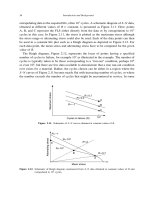
Figure 5.19. Smooth and notch fatigue data from [22] and methods for representing the notch curve.
It is often tempting to take a small amount of data that includes inherent scatter and
postulate a new or modified theory that will fit the data better than existing models. So,
not heeding my own advice, I offer the following as a method for fitting notch data based
on the results shown in Figure 5.19. Following the concepts presented above that were put

forth by Bell and Benham [18], the modification for the value of k
f
is further modified
slightly for the following reasons. If the notch behavior is purely elastic, then the value
of k
f
should not change for a given notch geometry. This region, on a Haigh diagram,
will cover values of mean stress from zero until the value at which the maximum stress,
S
max
, equals the yield stress, S
y
, or in terms of mean and alternating stress
S
m
=S
∗
m
when S
m
+S
a
=S
y
(5.16)
where S
∗
m
is defined as a transition mean stress. For values of S
m

below S
∗
m
, the fatigue
notch factor is constant and equal to the value of k
f
at R =−1, or zero mean stress,
which we denote by k
f0
. For mean stress values above S
∗
m
, we can allow the value of k
f
to
decrease linearly up to the ultimate strength, S
u
. This can be expressed by the equation,
which I will modestly call the “Nicholas equation,” as
k
f
=k
f0

1−
S
m
−S
∗
m

S
u
−S
∗
m

+
S
m
−S
∗
m
S
u
−S
∗
m
(5.17)
In the above, the transition mean stress is calculated from Equation (5.16) based on the
assumption that for a mild notch k
f
is approximately equal to k
t
. In reality, k
t
relates
the peak stress to the average stress so that k
t
will govern when first yielding occurs
Notch Fatigue 237

based on average stress values. Then, first yielding would occur as per Equation (5.16)
which is based on smooth bar values. The concept behind proposed Equation (5.17) is
that when the ultimate strength of the material with a notch is approached, the notch and
the smooth bar ultimate strengths are nearly the same because both involve net-section
yielding. Therefore, at the ultimate strength point, k
f
=1 for the notched specimen. The
linear variation is the simplest way to transition from the mean stress where yielding first
occurs to the ultimate strength. In the example shown in Figure 5.19, the value of k
f
is overestimated for data at high R when using a constant value of k
f
. If the “Nicholas
equation” (5.17) is used, as shown in Figure 5.20, the resulting curve, based on a Jasper
equation for representing the smooth bar data, produces an amazingly good fit to the
limited experimental data points. For this material, the yield strength was 135 ksi and the
transition mean stress S
∗
m
= 122ksi. While the fit to a limited data set in itself does not
completely prove or validate any such theory, the method has an advantage over using a
single value of k
f
. With a single value, the highest mean stress that can be predicted for
notch data is S
u
/k
f0
. Since smooth bar data are not available beyond a mean stress equal
to S

u
, the range in which predictions can be made is limited as shown in Figure 5.19
(also in Figure 5.20), where the constant k
f
equation terminates at a mean stress of under
75 ksi. The effect of using a constant value is to shrink the smooth bar curve radially
inward along lines of constant R on a Haigh diagram. It makes no sense to try to extend
the smooth bar equation to mean stresses beyond the ultimate strength. With the new
formulation, the notch curve is extended to the ultimate strength of the material without
having to extrapolate smooth bar data.
0
10
20
30
40
50
60
70
0 50 100 150
Smooth data
Notch data
Jasper Eqn
K
f
constant
Nicholas Eqn
Alternating stress (ksi)
Mean stress (ksi)
Ti-6Al-4V
k

t
= 2.5
k
f
= 2.0
UTS
Figure 5.20. Illustration of the proposed Nicholas equation ability to fit notch data.
238 Effects of Damage on HCF Properties
For the case of a straight-line modified Goodman equation used to represent smooth
bar data, this new approach would be equivalent to following the line called “brittle” in
Figure 5.11 from zero mean stress up to the transition mean stress, and then continuing
with a straight line to S
u
.
5.8.1. Negative mean stresses
Notched fatigue behavior for negative values of mean stress has received essentially no
attention in the open literature. With the recent increased usage of compressive residual
stresses for component fatigue life improvement, an increase in emphasis in this subject
can be expected. The use of surface treatments that produce compressive residual stresses
is discussed in Chapter 8. Here we discuss both uniform stress fields and those produced
by notches. In Figure 5.21, three possible methods of extrapolating the modified Goodman
equation
∗
into the negative mean stress region are shown. Each one is a straight line,
and the three lines are denoted by A, B, and C. There is no physical basis for any of
the three lines, but lacking data in the negative mean stress region, these three lines
cover a wide range of possible behavior in this region. For each of the lines, the notch
fatigue behavior is assumed to be governed by either of the two equations. First, the
fatigue notch factor is assumed to be linearly proportional to the mean stress so that
Mean stress

Alternating stress
0
A
B
C
A′
B′
C′
k
f
prop to mean stress
k

f
alt stress only
I′
I″
A″
B″
C″
S
0
S
0
/k
f
Figure 5.21. Representation of notch fatigue behavior for negative mean stress using three straight-line repre-
sentations of a Haigh diagram.
∗
The modified Goodman equation is a straight line from the value of the alternating stress at zero mean stress

to the ultimate stress at zero alternating stress.
Notch Fatigue 239
the value of k
f
goes from its reference value at R =−1 (zero mean stress) to unity at
the ultimate strength point in both tension and compression. This is equivalent to using
Equation (5.15) above with the added condition that S
un
= S
up
. The alternating stress at
zero mean stress is this s
0
/k
f
. These curves are denoted by A

,B

, and C

in the figure,
corresponding to the un-notched curves A, B, and C, respectively. The second method
of representing the notch fatigue behavior is to reduce only the alternating stress by the
same factor, k
f
, obtained (and defined) for R =−1. The curves for this condition are
denoted by A

,B


, and C

. In the positive mean stress region, the two methods produce
the same curve when the straight line is used to represent the un-notched behavior, as
pointed out earlier. In the negative mean stress region, a range of predicted behavior can
be seen. The wide variety of possible behavior, both for smooth and notched specimens,
provides a compelling argument for the generation of data in the negative mean stress
region before any meaningful modeling can be expected to be accomplished. At the time
of this writing, no such data have been found. This discussion is limited to relatively
blunt notches because the possibility of very sharp notches with small root radii closing
under compressive loading is a distinct possibility.
5.9. FATIGUE LIMIT STRENGTH OF NOTCHED COMPONENTS
An engineering approach to notches of arbitrary size and geometry which may or may
not have initial cracks has been developed by Hudak et al. [24]. It was developed to
explain the behavior of specimens subjected to FOD which can cause both craters and
cracks. It is based on a fracture-mechanics analysis using a concept similar to that of El
Haddad, et al. [12] described earlier, that attempts to predict the type of behavior shown
schematically earlier in this Chapter in Figure 5.6 where there are regions of growth to
failure, no initiation or growth, and an intermediate region of initiation but no growth.
The concepts are illustrated in Figure 5.22(a) where the regions of initiation and growth
to failure (A), initiation and arrest (B), and no initiation (C) are shown schematically.
The authors define a “worst case notch” as a value of k
t
, defined as K
w
, above which
further increase in k
t
no longer results in a decrease in threshold stress. In Figure 5.22(b),

the same regimes are shown as a function of crack size for a fixed value of notch depth
and different values of root radius. The upper and lower curves represent a large 
3

and small 
1
 root radius, respectively, while the horizontal line represents the limiting
radius, 
w
, corresponding to K
w
, above which crack arrest cannot occur (discussed earlier
in this chapter). What distinguishes this work from previous analyses is that the crack-size
effect is addressed by defining a crack-size dependent threshold in the form
K
th
a =K
th
R

a
a +a
0
(5.18)
240 Effects of Damage on HCF Properties
Stress concentration factor, K
t
σ
th
σ

th
Crack size, a
Threshold stress, ²
Δσ
e
/k
t
K
w
A
B
C
A
ρ
1
Crack arrest
(b)(a)
ρ
w
Crack growth
ρ
3
Crack growth
Figure 5.22. Schematic of regions of notch behavior.
where a
0
is the parameter defined by El Haddad in Equation (5.11) and K
th
is a function
of stress ratio, R. The curves shown in Figure 5.22(b) are generated for a specific geometry

and far-field loading by taking into account the actual stress field ahead of the notch and
calculating K as a function of crack length. The analysis allows for the prediction of
crack arrest or growth from a fracture-mechanics-based analysis and precludes the need
to use an empirical relationship for k
f
as a function of k
t
. It further has demonstrated that
the crack arrest which occurs at sharp notches depends both on the notch root radius and
depth, as well as on the crack and specimen geometry. The authors contend that simple
correlations between k
f
and k
t
are bound to break down for very deep, sharp notches
of the type that can be produced by FOD (see Chapter 7). This same type of analysis
can be used in contact fatigue problems (Chapter 6) where a complicated stress field,
involving steep stress gradients, is produced by the contact loading and not by sharp
notches. A further advantage over empirical approaches is that residual stresses, such
as those occurring during FOD, or those produced by surface treatments such as shot
peening, can be taken into account when calculating the stress intensity field ahead of
the notch.
The worst-case-notch concept has been extended to take into account local notch
plasticity. In addition, an approach that takes into account the surface area in the vicinity of
a notch, similar in concept to the critical volume or critical distance approaches to notches,
has been developed and is discussed later in this chapter. These two developments, that
were accomplished under a recently completed HCF program within the Air Force, are
described in detail in Appendix E.
Notch Fatigue 241
5.9.1. Non-damaging notches

One of the earliest attempts to quantify the size of a non-damaging notch, a notch that
does not reduce the fatigue limit strength of a material, is due to Lukas et al. [25]. Using
linear elastic fracture mechanics, they compared the stress intensity of an edge crack of
length l in a plate with that of a crack of the same length, l, emanating from an elliptical
notch having a notch root radius . For the former, the stress intensity is given as
K
plain
=112
√
l (5.19)
whereas for the crack from a notch, they used an approximation of results from FEM
analysis of Newman [26] in the form
K
notch
=
112k
t

√
l

1+45l/
(5.20)
where k
t
is the elastic stress concentration factor for the notch with root radius , and  is
the uniform far-field tensile stress. For both equations, a crack length l =l
0
is introduced
for which length the stress intensity is the threshold stress intensity for a long crack, and

the stress is the endurance limit stress for the smooth 
e
 and notched 
en
 specimens,
respectively. Applying their assumption that the depth of microcracks on the surface of
smooth specimens and the depth of microcracks at the notch root is the same at the fatigue
limit, Equations (5.19) and (5.20) are combined to produce the following formula for the
endurance limit at the notch,

en
=

e
k
t

1+45

l
0
/

(5.21)
From a large number of experiments on specimens having various radii, the best value of
l
0
was determined by trial and error fitting to Equation (5.21) for the FLS to be 100 m
for 15313 steel and 90m for copper.
The condition for a notch to be non-damaging with respect to the fatigue limit for the

same applied stress level and the same crack size l
0
 is shown to be

k
2
t
−1

 ≤45l
0
(5.22)
If Equation (5.19) is used to relate l
0
to the long crack threshold and the smooth bar
endurance limit, then l
0
becomes the same as a
0
in a Kitagawa diagram and the criterion
for a non-damaging notch takes the form

k
2
t
−1

 ≤114

K

th
/
e

2
(5.23)
This approach, which attempts to correlate the behavior of a notch with that of a smooth
bar, both of which have a crack, is essentially the same as using a Kitagawa diagram for
242 Effects of Damage on HCF Properties
the notch geometry (with a crack) and finding the crack length a
0
 where the endurance
limit and long crack threshold curve intersect. In this particular case, there is no El Haddad
small crack correction.
5.10. SIZE EFFECTS AND STRESS GRADIENTS
Continuing attempts have been made over the years to predict the fatigue limit of notched
components from data on smooth bars. The physical reasoning used has been that a critical
volume of material must be subjected to a critical stress level, the smooth bar fatigue
limit, in order for fatigue failure to occur. This postulate means that stress at a point,
for example at a notch root, is not the sole governing criterion for fatigue to occur. The
observations made that sharp notches have higher fatigue strengths than mild notches is
partial evidence for such a theory. Since the calculation of average stresses over a volume
is computationally intensive and impractical for many sharp notch geometries, the problem
is often simplified to one or two dimensions. This still would involve determination of the
average stress over some critical length. The simple solution for such a problem, adopted
by many, has been to use the stress at a critical distance from the surface to represent the
average stress over a larger distance. Critical volume approaches have been reviewed by
Sheppard [27] and Taylor and O’Donnell [28]. The empirical relations between k
f
and

k
t
, in many cases, are derived from determination of stresses over a critical length and
some simplifying assumptions about the distribution of stresses in order to come up with
a critical distance (see, for example, Peterson [4] who assumes a linear variation of stress
from the notch root).
5.10.1. Critical distance approaches
The critical distance approach has the advantage over many other empirical approaches
because it deals with both stress gradients and size effects. Taylor [13] shows, in fact, that
sharp notches and fatigue cracks have some commonality, as observed experimentally,
that the two behave similarly when the notch has a k
t
or sharpness beyond which the FLS
becomes coincidental with that of a crack of the same size. Taylor shows that the stress
determined at a critical distance a
0
/2, is the same for a sharp notch and a crack, where
a
0
is the length parameter of El Haddad determined from Equation (5.11). Numerical
results showing the stress distributions ahead of a circular notch of radius r, and of a
crack of length a, are shown in Figure 5.23, for three different values of a/a
0
; 0.1, 1.0,
and 10. The thick lines show the stress distribution for the notch, while the thin lines
represent that of the crack. The figure shows the overall distribution in (a), and a more
detailed distribution near the notch or crack tip, in (b). The vertical dashed line is the
location a
0
/2 which represents the location where the local stress determines the fatigue

Notch Fatigue 243
(a)
0
1
2
3
4
5
012345
Stress, σ/σ
0
r /a
0
Notch
a
/a
0
= 0.1
a
/a
0
= 1.0
a
/a
0
= 10
(b)
0
1
2

3
4
5
0 0.2 0.4 0.6 0.8 1
Stress, σ/σ
0
r /a
0
Notch
a
/a
0
= 0.1
a
/a
0
= 1.0
a /a
0
= 10
Figure 5.23. Numerical results showing the stress distributions ahead of a circular notch of radius, r, and of
a crack of length, a. Dashed line is at r =05a
0
. Plots (a) and (b) have different scales for r/a
0
.
strength based on smooth bar data at the same stress. As Taylor points out, for a very
sharp notch having a small radius, or a crack of the same length, the stresses at this point
are identical. For a large notch, the normalized stress approaches that corresponding to
the stress concentration factor which is three for the circular notch. Taylor also shows

244 Effects of Damage on HCF Properties
that the average stress over a length equal to 2a
0
provides the same numerical results
as the stresses at a point and, further, that the method produces the same prediction for
small crack behavior as that of El Haddad et al. [12] as given in Equation (5.11).
The critical distance concept for notch fatigue may involve quantities other than uniaxial
stress. Lanning et al. [21] review some approaches that involve use of a combination of
hydrostatic and shear stress and crack propagation thresholds. From a large body of notch
fatigue limit data generated on Ti-6Al-4V, they explored other quantities in a critical
distance approach to see if the data could be consolidated. In addition to evaluating
a quantity at a critical distance, they also used both an average value of a quantity
and a weighted average over some distance. Quantities evaluated included stress range,
mean stress, and elastic strain energy density. From FEM computations to obtain these
quantities for cylindrical notched specimens of varying notch depths and radii including
variations of applied stress ratio, R, some of which produced local notch plasticity, they
found best-fit parameters for each modeling concept. The use of a single critical distance
where the local stress range was evaluated produced the best overall correlation with the
experimental data. The authors conclude that the approach is moderately successful but
point out the difficulties that occur when local plasticity produces variations in R with
distance from the notch and when very small notch sizes are included in the database.
A further attempt to find a quantity that can be used to consolidate notch data with
smooth bar fatigue data using averaging over some critical distance was made by Naik
et al. [29]. Two approaches were used involving the Findley parameter, one was evaluating
the parameter at a critical distance, a
c
, and the other used the average value of the same
parameter over the same critical distance, a
c
. They used the Findley parameter, FIN, for

uniaxial stress in the form
FIN =
a
+k
max
(5.24)
where k is a fitting parameter and 
a
and 
max
are the maximum shear stress amplitude and
maximum normal stress on a critical plane that is defined as the plane where FIN is maxi-
mum. The parameter was shown to fit a large body of smooth bar fatigue data on Ti-6Al-4V
at several values of stress ratio, R, as illustrated in Figure 5.24 from [29]. For those data,
the best fit to the data is when the parameter has the form for an S–N type curve,
FIN =65739N
−06779
+4335N
−00415
(5.25)
To apply the parameter to notch data, the average value of the parameter over a distance
a
c
is called G
r
, and is given by
G
r
N =
1

a
c

a
c
0
FINx N dx =G
F
FIN
smooth
N (5.26)
where G
F
is defined as a notch gradient parameter. In this formulation, the critical
distance is not a material constant. Rather, the quantity G
F
is found to be a constant
Notch Fatigue 245
0
200
400
600
800
1000
10
3
10
4
10
5

10
6
10
7
10
8
10
9
R = –1
R = 0.1
R = 0.5
Curve fit
Findley parameter (MPa)
Cycles to failure
k = 0.29
Figure 5.24. Findley parameter for cycles to failure in Ti-6Al-4V from smooth bar data [29].
from calculations involving a wide range of notch geometries. With G
F
as a constant, a
quantity s is computed for any value of stress ratio, R, from
s =

1+

1−R
2k

2
(5.27)
where k is the constant in the Findley parameter, Equation (5.24). A quantity A

0
is
defined as
A
0
=

1+
2a
c


(5.28)
where  is the notch root radius and a
c
is the critical distance (not a constant). The authors
derive the relation

G
F
−2

A
0
2
+

G
F
s −1 +2s


A
0
−2s −1A
0
3/2
−G
F
s =0 (5.29)
from which A
0
can be calculated since G
F
is a material constant and s is obtained
from Equation (5.27) for any value of R. Once A
0
is found, the critical distance can be
obtained from Equation (5.28) and used in Equation (5.26) to obtain the value of FIN
from which number of cycles is determined using the equation that fits the smooth bar
data – Equation (5.25) in this example. The ability to consolidate notch data using this
approach is illustrated in Figure 5.25 where the constant G
F
= 116. This constant was
slightly different than the value of 1.21 obtained from a more limited set of notch fatigue
data, but the correlation was quite similar. For the results shown in Figure 5.25, the critical