High Cycle Fatigue: A Mechanics of Materials Perspective part 54 ppsx

516 Appendix C
envelope or within a larger population of engines. Frequency margin can be provided
above or below the steady-state speed. Engine components should not fail due to HCF
or a combination of HCF and LCF when subject to the maximum attainable combined
steady-state and vibratory stresses at a rate above that stated in A.4.13.3.
Low-order crossings and all known drivers within two stages either upstream or down-
stream of the subject component should have probabilistic design margins for final design
that account for the variation in speeds for different operating conditions. A deterministic
10% frequency margin on component modes is acceptable for preliminary design or when
there is insufficient confidence in probabilistic methods.
In the event that insufficient margin exists to meet the probability of failure requirement,
the next level of probabilistic design analysis is required. Such probabilistic design
analysis includes physical models of forced response, damping, and mistuning, along with
the appropriate probability models for each random variable and correlations between
those variables, as appropriate. Analyses on blades, vanes, disks, and integrally bladed
rotors (IBRs or blisks) should include the effects of response to unsteady aerodynamic
pressures, damping, and mistuning. Probabilistic methods should be applied to predict the
probability distribution of the dynamic responses. Without these analyses, HCF response
of the component may be seriously underestimated.
Appendix D
∗
Evaluation of the Staircase Test Method using
Numerical Simulation
Major Randall Pollak
INTRODUCTION
Numerical simulation was used to model the staircase test method for determining the
fatigue strength at a given number of cycles. The simulation allows the user to specify
the true fatigue strength distribution (modeled as normally distributed in all cases) by
specifying the mean and standard deviation of the fatigue strength at the number of cycles
of interest. Individual simulated test sequences for the staircase test procedure, described in
Chapter 3, are chosen randomly consistent with the assumed normal distribution function

and values of the parameters chosen for that function. Numerical simulation was used to
model the staircase test in order to determine the effects of starting stress, step size, and
number of specimens on parameter estimates using Dixon–Mood statistics as presented
in Chapter 3.
The objective of these simulations was to evaluate the feasibility of using the staircase
test to estimate a material’s fatigue strength distribution using small sample sizes. There
were two primary considerations when evaluating the staircase methodology. The first was
to assess how accurate the test is, on average. In this sense, the goal was to demonstrate
that the test method estimates the mean of fatigue strength distribution parameters as
closely to true values as possible—i.e., a test with little bias in results. The second
consideration involved the ability to estimate the scatter in results. Because a designer or
researcher must make conclusions based on a limited set of data, it is important that a
test should not be subject to a wide dispersion in results due to statistical scatter alone. In
other words, one would prefer a test method with results as tightly grouped as possible
around the true parameter values.
These two considerations led to recommending the use of two different techniques to
improve the fatigue strength analysis using a small-sample staircase test strategy. The first
technique involved the use of a non-linear correction term to the Dixon–Mood standard
deviation estimate in order to mitigate the bias inherent in this equation with small sample
∗
This document was prepared by Major Randall Pollak from the work that is part of his PhD dissertation at
the Department of Aeronautics and Astronautics, Air Force Institute of Technology. Much of the work in this
Appendix was presented at the 10th National Turbine Engine High Cycle Fatigue Conference in New Orleans,
LA, 8–11 March 2005.
517
518 Appendix D
sizes. The second technique was the incorporation of a simple bootstrapping algorithm to
help mitigate scatter in results. Through a combination of these techniques, a modified
staircase strategy emerged which is generally more accurate (less bias) and more precise
(less scatter) than traditional Dixon–Mood analysis alone.

THE STAIRCASE METHOD
The staircase method, first analyzed by Dixon and Mood [1] for explosives testing, and
later popularized by Little [2–3] for fatigue strength testing, utilizes a very simple protocol
in which a specimen is tested at a given starting stress for a specified number of cycles or
until failure, whichever occurs first. If the specimen survives, the stress level is increased
for the next specimen; likewise the stress is decreased if the specimen fails. This protocol
is continued for a batch of specimens with statistical equations applied to provide an
estimate for the mean fatigue strength and its standard deviation at the specified number
of cycles. Unfortunately, it is difficult in practice to provide accurate estimates of the
standard deviation using this method for small-sample test programs typical of high-cycle
or ultra high-cycle fatigue testing.
Typically, the step size between adjacent stress levels is held constant (approximately
equal to the standard deviation of fatigue strength), in which case the statistics of Dixon
and Mood may be applied directly to estimate mean and standard deviation of the fatigue
strength at a given number of cycles. Even though the true standard deviation in fatigue
strength is one of the unknowns, Dixon notes that it is not too important if the interval
is actually incorrect with respect to the true standard deviation by as much as 50% [4].
However, Little notes that arbitrary spacing between stress levels may be used when
accompanied by a probit-type analysis [2]. In fact, tests conducted with non-uniform
spacing may be more statistically efficient than uniform spacing; however, the analysis
becomes much more tedious and the equations and tables derived for uniformly spaced
tests are no longer useful [5].
The equations for the mean, , and standard deviation, , from the staircase method
(denoted by subscript “sc”) are (see Chapter 3):

SC
=S
i=0
+s
⎛

⎜
⎜
⎝
i
max

i=0
im
i
i
max

i=0
m
i
±05
⎞
⎟
⎟
⎠
(D.1)

SC
=162s
⎛
⎜
⎜
⎜
⎝
i

max

i=0
m
i
i
max

i=0
i
2
m
i
−

i
max

i=0
im
i

2

i
max

i=0
m
i


+0029
⎞
⎟
⎟
⎟
⎠
(D.2)
Appendix D 519
In these equations, s denotes the step size and the parameter “i” is an integer denoting
the stress level, with i
max
corresponding to the highest stress level in the staircase. If the
majority of specimens failed, then the lowest stress level at which a survival occurs (i.e.,
run-out) corresponds to the i = 0 level and m
i
corresponds to the number of specimens
which survived each stress level. The next highest stress level would be the i =1 level,
and the stress level one above that would be i = 2, etc. If the majority of specimens
survived the given number of cycles, then the lowest stress level at which a failure was
observed is denoted as the i =0 level and m
i
corresponds to the number of specimens
which failed at each stress level. The standard deviation equation above, Equation (D.2),
should only be used if the quotient term in this equation is greater than or equal to 0.3,
otherwise the standard deviation is estimated as 053s.
The primary condition of the analysis on which these equations is based is that the
variate under consideration must be normally distributed. In the case of fatigue testing,
this would imply that the fatigue strength distribution must be normally distributed.
This condition would seem to be very restrictive and rule out staircase testing for many

materials; however, a transformation of the stress values may be applied. For example,
the fatigue strength distribution of some materials may be reasonably represented using
a lognormal distribution, in which case the logarithm of stress values would be normally
distributed. The staircase test would then be conducted using steps of equal intervals with
respect to the natural logarithm of stress. Depending on the skewness of the distribution,
other transformations may be applied to make the distribution reasonably normal, although
there is no guarantee that every distribution can be transformed to approach normality. In
addition to logarithmic transformations, power transformations are often applied for such
a purpose. Squared and cubic transformations (as well as other powers greater than one)
are used to reduce negative skewness, while logarithmic and powers less than 1 (such
as a square-root transformation) as well as negative reciprocals (−1/x) are often used
to reduce positive skewness [6]. Thus, the normality condition is not as restrictive as it
first appears. However, it is often likely to be the case where there are not enough data
to actually estimate the distribution shape prior to conducting a staircase test. Thus, one
must either make a guess as to the shape based on data from a similar material and apply
an appropriate transformation if non-normal, or simply accept the initial assumption of
normality and conduct the test without a stress transformation and then use the data from
the experiment itself to estimate the distribution.
STAIRCASE SIMULATION
A computer simulation was designed to analyze the effects of staircase parameter settings.
The simulation allows the user to specify the true fatigue strength distribution (mean and
standard deviation). The underlying distribution was modeled as Gaussian in all cases.
520 Appendix D
The staircase test parameters (starting stress, step size, and number of specimens) were
then specified. For each specimen, the simulation calculated a random fatigue strength
based on the specified underlying distribution and compared this value to the current
stress level to determine if the specimen failed or survived. The stress level was then
increased or decreased for the next specimen according to the staircase protocol. This
procedure was repeated 1000 times in order to provide a distribution of calculated means
and standard deviations according to the Dixon–Mood equations. Comparison of runs

made with 1000 replications versus 10,000 replications showed that 1000 replications
provided more than adequate statistical significance. The simulation was later expanded
to allow the use of bootstrapping and various iterative test schemes.
STAIRCASE PARAMETER ANALYSIS
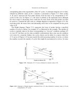
The first set of simulations focused on the effects of starting stress on parameter estimates
using the Dixon–Mood equations. Figure D.1a shows the effect of starting stress on
estimates of mean fatigue strength. Figure D.1b shows the starting stress impact on
standard deviation estimates.
As one would expect, starting higher than the true mean leads to an estimate for mean
fatigue strength that is slightly too high on average, and starting lower leads to lower
estimates. As the number of specimens increases, the importance of starting stress on
calculations of mean fatigue strength is diminished. This analysis reaffirms a fact that
is generally already accepted—namely, that one should start the staircase test as closely
to the true mean as possible. However, there are techniques already developed in the
literature to account for staircase results which begin with a string of failures (when
starting at stresses higher than the mean) or survivals (when starting too low). Brownlee
et al. first investigated this problem in 1953 and proposed a modified equation for the
mean [7]. Dixon later proposed a set of lookup tables for the mean in 1965 [4], and Little
expanded these tables in 1972 [5]. In short, there are adequate methods to estimate the
mean fatigue strength using small-sample data quite accurately.
For standard deviation estimation, Figure D.1b shows that even for small samples,
the effect of starting stress is rather small. However, use of offset starting stresses does
have some beneficial effect for small sample sizes by alleviating some of the standard
deviation bias. This result is due to the fact that when one starts above or below the
mean, it is statistically more likely that a failure will be observed below the mean (if
starting below) or a survival will be encountered above the mean (if starting above),
simply because one is conducting more testing above or below the mean, on average. In
a small-sample test, just one of these outcomes can lead to a higher estimate of standard
deviation, and therefore, on average, there is a slight reduction of the standard deviation
underestimating bias for small-sample tests. This effect is not overwhelming enough to

Appendix D 521
398.5
399.0
399.5
400.0
400.5
401.0
401.5
0 50 100 150 200
0 50 100 150 200
Number of specimens
Point estimate of FS mean
Start at mean
Start 2 steps below
Start 2 steps above
2
3
4
5
6
Number of specimens
Point estimate of FS standard deviation
Start at mean
Start 2 steps below
Start 2 steps above
(a)
(b)
Figure D.1. Effect of starting stress on (a) mean and (b) standard deviation estimates for true underlying
distribution Normal ( =400 =5) and step size 1.
eliminate the bias altogether, but does provide some means of softening it. For the data in

Figure D.1b, the mean standard deviation for N =10 samples is 3.68 (26.3% error) when
starting at the mean, but 4.06 (18.9% error) when starting two steps below the mean. The
traditional approach of starting the staircase at the mean in order to maximize accuracy
of the estimate for mean fatigue strength may be modified in order to improve standard
522 Appendix D
deviation estimation, especially since adequate means of handling offset starting stresses
exist for mean fatigue strength estimation.
Next, the effect of step size was analyzed. The choice of step size had little effect on
the calculated fatigue strength mean in an average sense, although Figure D.2 shows that
as step size increases, there is more scatter in fatigue strength mean estimates. This result
is rather intuitive since one would expect a tighter grouping around the mean for small
steps. Thus, a single staircase test is more likely to have error in calculated mean fatigue
strength for larger steps versus smaller steps.
Figure D.3 shows the calculated standard deviation as a function of step size and
number of specimens. This figure represents the expected value of standard deviation for
any combination of step size and number of specimens. When normalized by the true
standard deviation, these expected values are independent of the true standard deviation.
Note that in the limit (simulated using 1000 specimens), the calculated standard deviation
is close to the true standard deviation for all step sizes ranging from 01 to 17.
However, for small-sample tests, the standard deviation is significantly underestimated.
Braam and van der Zwaag [8], along with Svensson and de Maré [9], also noted this
underestimating bias for small-sample tests. Note that existing guidance stemming from
Dixon and Mood’s original work suggests a step size in the 2/3to3/2 range. To
remove standard deviation bias, however, Figure D.3 shows that step sizes must be larger,
on the order of 16 to 175. Beyond this region, the standard deviation estimates
converge to the 053s line. It is clear from Figure D.3 that standard deviation bias is
magnified as either step size or sample size are reduced.
0.0
0.5
1.0

1.5
2.0
2.5
3.0
0 0.5 1 1.5 2
Step size (σ)
Standard deviation of FS mean
8 specimens
10 specimens
12 specimens
15 specimens
20 specimens
30 specimens
50 specimens
100 specimens
1000 specimens
Figure D.2. Effect of step size on scatter of fatigue strength mean estimates for true underlying distribution
Normal ( =400 =5).
Appendix D 523
0.0
0.1
0.2
0.3
0.4
0.5
0.6
0.7
0.8
0.9
1.0

1.1
1.2
0 0.5 1.5 2
Step size (σ)
Point estimate of standard deviation (σ)
8 specimens
10 specimens
12 specimens
15 specimens
20 specimens
30 specimens
50 specimens
100 specimens
1000 specimens
1
Figure D.3. Effect of step size on estimated fatigue strength standard deviation.
In addition to being more accurate on average, use of a higher step size reduces the
variance in standard deviation estimates compared to the estimates obtained using a step
of 2/3to3/2, as illustrated by Figure D.4. This effect is due in part to the larger steps
producing more results using the 053s standard deviation estimate, which is constant for
a given step size. In general, it appears that use of steps in the 16 to 175 range will
result in both less bias and less scatter than smaller step sizes.
0.0
0.1
0.2
0.3
0.4
0.5
0 0.5 1 1.5 2
Step size (σ)

Standard deviation of D–M (σ)
8 specimens
10 specimens
12 specimens
15 specimens
20 specimens
30 specimens
50 specimens
Figure D.4. Effect of step size on scatter of fatigue strength standard deviation estimates.
524 Appendix D
Thus, there is a bit of a tradeoff here. Larger step sizes on the order of 17 provide
generally more accurate estimates of standard deviation with less scatter, but result in
slightly more scatter in fatigue strength mean. Remedies to this tradeoff will be presented
in the next section.
CORRECTION FOR STANDARD DEVIATION
Due to the bias in standard deviation estimates for small sample sizes, a correction term
was investigated to allow the use of Dixon–Mood equations at smaller steps to avoid the
increased scatter in fatigue strength estimates inherent in the use of higher step sizes. A
starting point for such a correction was the linear correction factor presented by Svensson
et al. [10]. This work addressed the problem of standard deviation bias, noting that no
theoretical solution to this bias was apparent. A correction factor for the standard deviation
was proposed based on the number of tested specimens, given as:

corr
=
DM

N
N −3


(D.3)
where 
corr
is the modified (corrected) standard deviation, 
DM
is the standard deviation
calculated using the Dixon–Mood equation, and N is the number of specimens.
This linear correction (which will be called the “Svensson–Lorén correction” herein)
was applied to the standard deviation estimates from the simulation results from
Figure D.3, with corrected standard deviations shown in Figure D.5. Notice that the step
0.0
0.2
0.4
0.6
0.8
1.0
1.2
1.4
1.6
1.8
0 0.5 1.5 2
Step size (σ)
Correction of mean standard deviation (σ)
8 specimens
10 specimens
12 specimens
15 specimens
20 specimens
30 specimens
50 specimens

100 specimens
1000 specimens
1
Figure D.5. Svensson–Lorén correction for fatigue strength standard deviation estimates.
Appendix D 525
size for unbiased standard deviation estimates has shifted from 17 to approximately
1. This result is significant since it allows the use of smaller step sizes without standard
deviation bias. However, since the true standard deviation is unknown, it is not possible
to plan a test at precisely this unbiased step size. If one tests at too low a step size,
standard deviation is still underestimated (on average). Likewise, the standard deviation
is overestimated at higher step sizes. One would prefer a correction which allowed a
greater range of unbiased step sizes.
A more elaborate correction factor was developed based on analysis of simulation
results and is proposed for small-sample staircase tests. This correction factor accounts
for both sample size and step size, and has the form:

corr
=A
DM

N
N −3


B

DM
s

m

(D.4)
In this equation, A B, and m are constants based on the number of specimens, with
other variables as previously defined. Table D.1 shows the values for these constants
based on simulation results for selected numbers of specimens. Since standard deviation
bias is independent of both the true mean and true standard deviation of the underlying
fatigue strength distribution, these constants are not specific to a particular simulation
case. These constants were determined in order to calibrate the mean standard deviation
estimate from Dixon–Mood analysis to be as unbiased as possible. Figure D.6 shows
the corrected mean estimates for standard deviation using this non-linear correction, with
Figure D.7 comparing the standard deviation estimates for Dixon–Mood, the Svensson–
Lorén correction, and this non-linear correction for N = 20 specimens.
These figures suggest that the proposed correction allows a greater range of unbiased
(or only slightly biased) step sizes. Thus, when using this correction, one is less reliant on
the initial guess of true standard deviation in order to get meaningful results. However,
it should be noted that it is only the mean standard deviation from Dixon–Mood that is
Table D.1. Non-linear correction constants
based on number of specimens
Number of specimens AB m
8 1.30 1.2 1.72
10 1.08 1.2 1.10
12 1.04 1.2 0.78
15 0.97 1.2 0.55
20 1.00 1.2 0.45
30 1.00 1.2 0.22
50 1.00 1.2 0.15
>50 Use Svensson–Lorén.