High Cycle Fatigue: A Mechanics of Materials Perspective part 64 docx

616 Appendix H
is provided, it shall be demonstrated once during each shut down. Components such as
air-oil coolers with exposure to inlet sand and dust conditions shall be considered inlets for
this test but a rig test may be performed to satisfy the requirements herein. Following the
post-test performance check, the engine shall be disassembled to determine the extent of
sand erosion, and the degree to which sand may have entered critical areas in the engine.
The test will be considered satisfactorily completed when the criteria of 3.3.2.4 have been
met and the teardown inspection reveals no failure or evidence of impending failure.”
Background:
The recommended text decreases the operational time in the extreme sand and dust
environment from ten hours to two hours for turbofan and turbojet engines. Engine
contractors have been unwilling in the past to guarantee their engines for ten hours
(helicopter subjected to the severe Vietnam sand and dust environment typically used
inlet filtration systems). The time requirement will have to be negotiated with each engine
contractor in specific future specification negotiations based upon the intended usage in
regions of the world where sand will be a concern.
The sand concentration should be calculated with customer bleed air extraction. The
anti-icing switch should be activated five times during each hour of sand ingestion at
equally spaced intervals. The test should be conducted with a thrust bed and load cell
measurement of thrust in lieu of calculating thrust by EPR. Disassembly and inspection
between the coarse and fine sand tests should be conducted for 45.4 kg/s (100 lb./sec)
airflow or smaller engines.
VERIFICATION LESSONS LEARNED (A.4.3.2.4)
The Engine V sand and dust test did not use the recommended sand and dust mixture
due to commercial unavailability of the mixture. The specification for fine sand calls for
a particle size distribution which cannot be obtained commercially. Specifically, calcite
and gypsum could not be obtained with a particle size distribution to match the specified
particle size distribution. Table XXXVIa and b shows the closest particle size distributions
which the Engine V sand and dust test team could find along with the required size
distribution.
Appendix I

∗
Computation of High Cycle Fatigue Design Limits
under Combined High and Low Cycle Fatigue
Joseph R. Zuiker
ABSTRACT
Applications in rotating machinery often result in stress states that produce both low cycle
fatigue (LCF) damage in addition to the damage produced from the high frequency or
high cycle fatigue (HCF) vibratory loading. While the Haigh diagram takes into account
the vibratory as well as the steady stress amplitudes for a fatigue limit corresponding to
a (large) given number of cycles, it does not consider the combined effects of LCF and
HCF. To account for the combined effects analytically, an initiation model for combined
cyclic fatigue (CCF) is coupled with a threshold fracture mechanics crack propagation
model to predict fatigue thresholds for CCF. The results are contrasted with the HCF
allowable stresses represented in a constant-life Haigh diagram. Experimental data from
the literature for a Ti-6Al-4V alloy are used to demonstrate the viability of the analysis
and the limitations of the use of the Haigh diagram in design. Comments on the limitations
on the use of a Haigh diagram for combined HCF–LCF loading are presented.
NOMENCLATURE
C Paris-Walker law constant
CCF combined cycle fatigue
d Paris-Walker law constant
d damage parameter
d
i
initiation phase damage parameter
D diameter of rod
HCF high cycle fatigue
K
t
stress concentration factor

LCF low cycle fatigue
LEFM linear elastic fracture mechanics
∗
This document was contributed by Dr. Joseph Zuiker, a former employee of the Air Force Research Laboratory.
It is based on unpublished work conducted by him while with the Air Force. Dr. Zuiker is currently with
General Electric Company Power Systems Division.
617
618 Appendix I
m Paris-Walker law constant
n number of HCF cycles per LCF cycle
N number of CCF cycles
N
iCCF
number of cycles to crack initiation in CCF loading
N
iHCF
number of cycles to crack initiation in HCF-only loading
N
iLCF
number of cycles to crack initiation in LCF-only loading
Q stress intensity range ratio =K
HCF
/K
LCF
r exponent for initiation life equation
R stress ratio =
min
/
max
 crack growth rate acceleration factor

K
HCF
stress intensity factor range of HCF cycles
K
LCF
stress intensity factor range of LCF cycles
K
th
threshold stress intensity factor range
K
onset
K
LCF
value at which HCF crack growth becomes active in CCF
K
tho
K
th
at R =0 (in CTOD-based model)

HCF
strain range of HCF cycle
 stress range

end
endurance limit stress range below which no initiation damage is caused

HCF
stress range of HCF cycle


LCF
stress range of LCF cycle

∗
constant for initiation life equation

a
alternating stress

aeq
equivalent alternating stress at R =0 for a stress state at R =0.

aHCF
alternating stress of HCF cycle to be converted to equivalent R =0 cycle

fs
alternating stress causing failure in a specified number of cycles at R =−1

m
mean stress

mHCF
mean stress of HCF cycle to be converted to equivalent R =0 cycle

ult
ultimate strength

y
yield strength
INTRODUCTION

Design of components for HCF must generally account for the detrimental effects of a
superimposed mean stress. This accounting is often in the form of an alternating versus
mean stress (Haigh) diagram that shows allowable vibratory stress amplitude as a function
of applied mean stress for a specified life. In many cases little or no data are available for
conditions other than fully reversed loading where the stress ratio R = 
min
/
max
=−1,
and tensile overload R = 1 or ultimate stress, and assumptions such as a straight line
fit must be made in order to interpolate between these limiting cases.
Appendix I 619
A more general Haigh diagram can be produced using data at various values of mean
stress and a specified number of cycles to failure, e.g. 10
7
, as obtained from S–N curves
and plotting the locus of points. For any of these plots, the number of cycles is typically
taken to be those corresponding to a “runout” condition, perhaps 10
8
or even 10
9
, but
there are few data available to demonstrate that a true runout condition ever exists for a
material. This has been shown to be the case in several studies on titanium (cf. [1, 2]).
For convenience and practicality, the number of cycles chosen is taken to correspond to
the region where the S–N curve becomes nearly flat with increasing number of cycles,
or is selected such that the number of cycles exceeds that which might be encountered in
service. In some cases, neither condition may be satisfied. For design purposes, because
of the statistical variability of fatigue data, particularly in the long-life regime where S–N
curves tend to be close to horizontal, Haigh diagrams commonly represent a statistical

minimum. For the purposes of the present discussion, only average material property data
will be discussed.
The straight line Goodman assumption and corresponding Haigh diagram are widely
used in design for HCF. Henceforth, we shall consider only the Goodman assumption, but
it is understood that any discussion of the Haigh diagram is equally valid for any other
assumptions regarding the shape of the diagram. A critical issue in the use (or misuse) of
the Haigh diagram in design is the degree of initial or service induced damage that may
be present in a component, but may not be present in the material used for generation of
the Haigh diagram. In the present study, we deal with damage induced by superimposed
LCF. If such damage is present, the Haigh diagram is not valid for the material because
it represents “good” or undamaged material. Therefore, a design methodology which
considers the development of damage from sources other than the constant amplitude
HCF loading must be used to account for the different state of the material. Turbine
engine components, for example, which are subjected to HCF, are typically subjected to
LCF in addition because the non-zero mean stress is achieved through the centrifugal
loading typical of operation. Each startup and shutdown constitutes an LCF cycle. Thus,
the component experiences combined HCF and LCF or CCF and, for design purposes,
the effect of LCF loading on the HCF life should be considered.
In this appendix, we present a simple model for the CCF of a typical turbine engine
alloy and use data from the literature to predict the effect of superimposed LCF on the
HCF capability of the material. Here, LCF refers to large amplitude, low frequency cycles
whose total number is typically less than 10
3
–10
4
, while HCF refers to small amplitude,
high frequency cycles at high mean stress, whose number generally exceeds 10
6
–10
7

.
In the following sections, a prediction methodology is described including descriptions
of the initiation life model, the propagation life model, the experimental data used to
calibrate the model, and the assumptions concerning the interaction of the HCF and LCF
cycles. Then, numerical predictions are presented to confirm the model accuracy and
620 Appendix I
show its sensitivity to a variety of factors. Finally, we close with a discussion of the
results, conclusions, and possible future efforts.
It is important to note a principal difference between this work and the majority of the
previous studies on CCF. While most of the literature has been concerned with the effect
of superimposed HCF on the LCF life of materials and structures, this appendix deals
with the effect of superimposed LCF on the HCF capability of the material and further
and, further, addresses total life as a sum of initiation and propagation phases, the latter
of which uses fracture mechanics analysis.
LIFE PREDICTION METHODOLOGY
In order to illustrate HCF–LCF interactions, analytical predictions are made of the total
fatigue life and presented as a Haigh diagram for a material experiencing 10
7
HCF cycles
divided equally over N LCF loading blocks. It is assumed that total life can be divided
into two distinct phases: a crack initiation phase, and a crack propagation phase. Each
CCF loading block consists of a low frequency cycle over which the material is loaded
from zero stress to a given mean stress and held while n=10
7
/N high frequency cycles
are superimposed about the mean stress as shown schematically in Figure I.1. The details
of the analysis follow.
Initiation life
During initiation the material is assumed to be uncracked. Initiation damage, d
i

,is
accumulated over each HCF and LCF cycle until d
i
=1 at which point it is assumed that
a crack of depth a
i
has initiated. The number of LCF cycles required to reach d
i
=1is
σ
m
σ
a
2
σ
LCF
2
σ
HCF
Time
n
= 8
Stress (strain)
ONE CCF LOAD BLOCK
Figure I.1. Idealized combined cycle fatigue load block.
Appendix I 621
defined as N
iLCF
. For LCF-only cycling applied at R =0  =2
a

=2
m
, a power law
function of the applied stress range using a form similar to the Basquin equation is used
such that
N
iLCF
=
∗
2
a

r
(I.1)
where 
a
is the alternating stress amplitude and 
∗
and r are constants. In fitting the
response of actual materials, multiple sets of constants are used over specific ranges
of 
a
such that Equation (I.1) forms a piece-wise linear approximation to the actual
material response when plotted on a log-log scale. Equation (I.1), which is written for
LCF-only loading R =0, can also be used for HCF cycles at R =0 by substituting an
equivalent alternating stress amplitude, 
aeq
. The equivalent alternating stress is obtained
by moving along a line of constant life on a Haigh diagram from the point defining the
HCF cycle 

m

a
 at R = 0 to a point at R = 0. The form of the constant life line
must be assumed. Here, we postulate that the straight-line Goodman assumption governs
mean stress effects on initiation life in the same manner as it governs mean stress effects
on total life. That is, straight lines passing through 
ult
 0 exhibit constant initiation
life. The fully reversed stress to initiation, 
fsi
is defined as the y-axis intercept of a
line passing through points defining the HCF load cycle at R = 0 
mHCF
, 
aHCF
 and

ult
 0. Fully reversed initiation stress, 
fsi
can be defined in terms of 
aHCF
, 
mHCF
,
and 
ult
; and substituted into the modified Goodman equation for 
fs

, the fully reversed
alternating stress amplitude. The equivalent alternating stress is then obtained by setting

a
=
m
=
aeq
and solving for 
aeq
,as

aeq
=
1

1

ult
+
1

aHCF
−

mHCF

aHCF

ult


(I.2)
Thus, the initiation life due to HCF cycles, N
iHCF
, is obtained via Equation (I.1) by
replacing 
a
with 
aeq
from Equation (I.2).
To determine the initiation life under combined HCF–LCF loading, the linear damage
summation model [3, 4] is used such that the initiation life, in CCF blocks, is
N
iCCF
=
1

1
N
iLCF
+
n
N
iHCF

(I.3)
where N
iCCF
is the initiation life under CCF in terms of CCF load blocks. The linear
damage summation model has been criticized for its inability to account for load sequenc-

ing affects. However, it is noted that when different cycles are mixed evenly over the
life of a component, the Palmgren–Miner rule gives acceptable results (cf. [5, 6]). More
advanced nonlinear damage summation models have been proposed. While many give
622 Appendix I
better results than the linear damage summation model, they are often limited to specific
materials or conditions and require experience to be used with confidence [7].
After N
iCCF
loading blocks, a crack, which is amenable to fracture mechanics techniques
for predicting crack growth, is assumed to have formed in the component and grows
according to LEFM to failure. The size, shape, and location of the crack must be assumed
and, here, will be taken from experimental data in the literature.
For cases in which N
iCCF
1, it may be sufficiently accurate to round N
iCCF
to the nearest
integer and begin crack propagation with the next load block. In other cases this may not be
accurate and itis important to determine atwhat point in theload block the crackinitiates and
crack propagation begins. As a first approximation, it is assumed thatall initiation damagein
each cycle occurs duringthe loading portion of thecycle. Thus, if N
iCCF
is fractional, the first
portion of the fractional cycle is attributed to the LCF cycle; the remainder of the fractional
initiation damage is attributed to HCF cycles, and during the remaining portion of the load
block the crack is assumed to have initiated and begins to grow in HCF.
Initiation example
Consider the case of a specified loading sequence consisting of n = 8000 HCF cycles per
CCF load block. For a specified maximum stress and HCF stress range, the initiation lives
are found as N

iLCF
=16×10
4
and N
iHCF
=3×10
7
. In this case, the initiation damage per
CCF load block due to LCF is d
iLCF
=1/N
iLCF
=6250 ×10
−5
, the initiation damage per
CCF load block due to HCF is d
iHCF
=n/N
iHCF
=2667×10
−4
, the total initiation damage
per CCF load block is d
iCCF
=d
iLCF
+d
iHCF
=3292 ×10
−4

, and N
iCCF
=1/d
iCCF
=
3037975. Thus, after 3037 CCF load blocks, d
i
=0999679. During the loading portion
of the LCF cycle in load block 3038, d
i
increases by 6250 ×10
−5
to 0999742 ×10
−n
.
Each HCF cycle then increases the damage by 3333 ×10
−8
until the crack initiates after
7740 HCF cycles in load block 3038. Thus, during HCF cycle 7741 in CCF load block
3038, the crack is considered to have initiated and begins to grow under the assumptions
of fracture mechanics.
Propagation life
During the crack propagation phase, the crack grows under the assumptions of linear
elastic fracture mechanics. Short crack behavior is neglected. During LCF and HCF
cycles, the crack is assumed to grow in mode I following the Paris law as modified by
Walker [8] to account for stress ratio effects as
da
dN
∗
=C

K
m
1–R
d
(I.4)
Here, C and m are material constants describing the crack growth rate at R=0, and d is
a material constant accounting for the higher crack growth rate at higher R for the same
Appendix I 623
K, an effect attributed to K
max
or mean stress effects. For LCF cycles, N
∗
corresponds
to a single LCF cycle, K
LCF
replaces K, and R=0. For HCF cycles, N
∗
corresponds
to a single HCF cycle, K is replaced by K
HCF
, and in general R>0. Equation (I.4)
holds for K>K
th
for individual LCF cycles as well as individual HCF cycles provided
that the appropriate stress range and value of R are used in each case. In accordance with
experimental observations, K
th
is assumed to be a decreasing function with increasing
R. The values of K
LCF

and K
HCF
are calculated from 
LCF
and 
HCF
which are
shown in Figure I.1. It can be deduced from the figure that K
HCF
is typically less than
K
LCF
for a given crack length and, therefore, the threshold in LCF should be reached
before that in HCF. However, when considering growth rate per block of cycles, the
number of cycles per block, n, if large, could dominate the growth rate if both values of
K for HCF and LCF are above threshold.
In the case of tension–compression cycling R<0, the crack tip is assumed to be
open, and the crack growing, only when the applied stress is positive. Thus, the minimum
effective stress is always positive or zero, and R never drops below zero in Equation (I.4).
This is, however, a minor point as we are most interested in loading typical of turbine
engine components in which the mean stress is high, the vibratory stress is relatively low,
and R
HCF
>0.
The specimen is assumed to fail when K
max
surpasses K
IC
, or when the crack depth
exceeds an appropriate length scale indicative of tensile overload in the specimen,

whichever occurs first. Crack growth is calculated for each HCF and LCF cycle, and is
assumed to occur during the loading portion of each cycle. Thus, growth increments are
determined sequentially for an LCF cycle, n HCF cycles, another LCF cycle, and so on.
Under these assumptions, several failure sequences are possible. The particular
sequence encountered is a function of four characteristic crack depths that, in turn, are a
function of the material properties and LCF and HCF stress ranges. They are
•
a
i
– the crack depth at initiation, which is defined by experimental data
•
a
crit
– the crack depth at which K
IC
is exceeded at the crack tip (or a depth appropriate
to the specimen size if a
crit
exceeds characteristic specimen dimensions), which is a
function of 
HCF
, 
LCF
, and K
IC
•
a
gLCF
– the crack depth beyond which the crack grows during LCF cycles, which is
a function of 

LCF
and K
th
(at R=0 for LCF cycles) and
•
a
gHCF
– the crack depth beyond which the crack grows during HCF cycles, which is
a function of 
HCF
and K
th
(at R for HCF cycles).
There are 24 possible permutations of these four crack depths, any of which will produce
one of seven failure sequences which are shown in Figure I.2. Path 1 is not likely if
reasonable initiation data are available. Path 2 is unlikely for load levels of interest. Paths
4 and 7 produce HCF-only crack propagation, which is a possible failure mode if K
th
in HCF (at high R) is sufficiently small in comparison with K
th
in LCF (at R=0),
624 Appendix I
a
crit

≤

a
i

?
1) Fast fracture immediately
after initiation
a
i
< a
g,

HCF
and a
i
< a
g,

LCF
?
a
i
≥ a
g,

HCF
and a
i
≥ a
g,

LCF
?
a

crit
≥ a
g, LCF
and a
i
≥ a
g,

HCF
?
a
crit
≥ a
g,

HCF
and a
i
≥ a
g,

LCF
?
2) No propagation after
initiation. Infinite life
3) Initiation followed by crack
growth in CCF to failure
4) Initiation followed by crack
growth in HCF only to failure

5) Initiation followed by crack
growth in LCF only to failure
a
crit
> a
g,

HCF
and a
g,

HCF
≥ a
i
and a
i
≥ a
g,

LCF
?
6) Initiation followed by crack
growth in LCF only followed by
crack growth in CCF to failure
7) Initiation followed by crack
growth in HCF only followed by
crack growth in CCF to failure
Yes
Yes
Yes

Yes
Yes
Yes
No
No
No
No
No
No
Figure I.2. Flow chart of possible failure sequences under CCF.
and 
HCF
is sufficiently large to grow the crack. While this situation depends on the
assumed relation of K
th
with R, neither of these HCF-only crack propagation modes
has been observed in any of the numerical calculations reported here. Paths 3, 5, and 6,
then, are of the most practical interest.
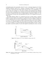
Model Calibration
In order to calibrate and exercise the model, crack initiation and propagation data on
surface-cracked round bars [9] are used. In this study, electropotential drop techniques
were used to determine the number of cycles required to produce 50m deep surface
Appendix I 625
cracks in mildly notched K
T
=2 Ti-6Al-4V round bars with an / microstructure.
Total life was measured in both mildly notched and smooth bars. Chesnutt et al. [10]
and Grover [11] reported total life measurements on Ti-6Al-4V materials with a similar
microstructure at lower stress levels (and longer lives) at various values of K
T

. Using
these data, total life estimates for long life tests at K
T
=2 were interpolated and are
shown, along with the short life data by Guedou and Rongvaux [9], in Figure I.3. A
multi-part power law fit to the initiation life curve was generated by connecting the
ultimate stress at N =1 to the LCF data from Guedou and Rongvaux [9]. A power law
fit to the experimental data was extrapolated to lower stress values. Two scenarios were
considered for low stresses. In the first, alternating stress ranges below 300MPa R=0
cause no damage. Thus the life is infinite for lower stresses and the final portion of the
S–N curve is a horizontal line. This stress range was chosen to agree approximately with
the observed runout behavior in the long life tests [10, 11]. The contrasting scenario
assumes that no endurance limit exists. Any alternating stress causes a finite amount of
damage. In this scenario, the S–N curve extends downward continuously. Both cases
are shown in Figure I.3. The corresponding total life curve was generated by adding the
analytical estimate of the propagation life to the initiation life measurement and correlated
well with the experimentally measured total life values shown in Figure I.3.
Crack propagation data at R =005 and 0.85 [9] were used to determine parameters
C, m, and d for the Paris–Walker relation in Equation (I.3). The values used here are
C =5376 ×10
−12
, m=3409, and d=13. The values of K
th
for Ti-6A1-4V are taken
10
3
10
4
10
5

10
6
10
7
200
300
400
500
600
700
800
900
1000
N
I
K
t
=

2 (Guedou and Rongvaux, 1988)
N
T
K
t
=

2 (Guedou and Rongvaux, 1988)
N
T
K

t
=

1 (Chessnutt et al., 1978)
N
T
K
t
=

3.4 (Chessnutt et al., 1978)
N
T
K
t
=

2 (Interpolated)
N
I

K
t
=

2 (Predicted)
N
T
K
t

=

2 (Predicted)
N
Stress range (MPa)
ENDURANCE LIMIT: 2 σ
a
= 300 MPa
NO ENDURANCE LIMIT
Figure I.3. Predicted and measured values of N
i
and total life N
T
 as a function of applied stress range
at R=0.