Commodity Trading Advisors: Risk, Performance Analysis, and Selection Chapter 8 pot

PART
Two
Risk and Managed
Futures Investing
Chapter 8 uses a unique data set from the Commodity Futures Trading
Commission to investigate the impact of trading by large hedge funds and
commodity trading advisors (CTAs) in 13 futures markets. Regression
results show there is a small but positive relationship between the trading
volume of large hedge funds and CTAs and market volatility. Further results
suggest that trading by large hedge funds and CTAs is likely based on pri-
vate fundamental information.
Chapter 9 examines the dynamic nature of commodity trading programs
that tend to mimic a long put option strategy. Using a two-step regression
procedure, the authors document the asymmetric return stream associated
with CTAs and then provide a method for calculating value at risk. The
authors also examine a passive trend-following commodity index and find
it to have a similar put optionlike return distribution. The authors also de-
monstrate how commodity trading programs can be combined with other
hedge fund strategies to produce a return stream that has significantly lower
value at risk parameters.
Chapter 10 examines the relationships between various risk measures
for CTAs. The relationships are extremely important in asset allocation. If
two measures (e.g., beta and Sharpe ratio) produce identical rankings for a
sample of funds, then the informational content of the two measures are
similar. However, if the two measures produce rankings that are not identi-
cal, then the informational content of each measure as well as asset alloca-
149
c08_gregoriou.qxd 7/27/04 11:13 AM Page 149
tion decisions may be unique. Interdependence of risk measures has been
examined previously for equities and recently for hedge funds. In this chap-
ter the authors analyze 24 risk measures for a sample of 200 CTAs over the

period January 1998 to July 2003.
Chapter 11 provides a simple method for measuring the downside pro-
tection offered by managed futures. Managed futures are generally consid-
ered to help reduce the downside exposure of stocks and bonds. The
chapter also measures the downside protection provided by hedge funds
and passive commodity futures indices. In each case, considerable downside
protection is offered by each of these three alternative asset classes.
8
150 RISK AND MANAGED FUTURES INVESTING
c08_gregoriou.qxd 7/27/04 11:13 AM Page 150
CHAPTER
8
The Effect of Large Hedge Fund
and CTA Trading on Futures
Market Volatility
Scott H. Irwin and Bryce R. Holt
T
his study uses a unique data set from the CFTC to investigate the impact
of trading by large hedge funds and CTAs in 13 futures markets. Regres-
sion results show there is a small but positive relationship between the trad-
ing volume of large hedge funds and CTAs and market volatility. However,
a positive relationship between hedge fund and CTA trading volume and
market volatility is consistent with either a private information or noise
trader hypothesis. Three additional tests are conducted to distinguish between
the private information hypothesis and the noise trader hypothesis. The first
test consists of identifying the noise component exhibited in return variances
over different holding periods. The variance ratio tests provide little support
for the noise trader hypothesis. The second test examines whether positive
feedback trading characterized large hedge fund and CTA trading behavior.
These results suggest that trading decisions by large hedge funds and CTAs

are influenced only in small part by past price changes. The third test con-
sists of estimating the profits and losses associated with the positions of large
hedge funds and CTAs. This test is based on the argument that speculative
trading can be destabilizing only if speculators buy when prices are high and
sell when prices are low, which, in turn, implies that destabilizing specula-
151
The authors thank Ron Hobson, and John Mielke of the Commodity Futures Trad-
ing Commission for their assistance in obtaining the hedge fund and CTA data and
answering many questions. This chapter is dedicated to the memory of Blake Imel
of the CFTC, who first suggested that we analyze the hedge fund and CTA data and
provided invaluable encouragement. We appreciate the helpful comments provided
by Wei Shi.
c08_gregoriou.qxd 7/27/04 11:13 AM Page 151
tors lose money. Across all 13 markets, the profit for large hedge funds and
CTAs is estimated to be just under $400 million. This fact suggests that trad-
ing decisions are likely based on valuable private information. Overall, the
evidence presented in this study indicates that trading by large hedge funds
and CTAs is based on private fundamental information.
INTRODUCTION
In recent years, hedge funds and commodity trading advisors (CTAs) have
drawn considerable attention from regulators, investors, academics, and the
general public.
1
Much of the attention has focused on the concern that
hedge funds and CTAs exert a disproportionate and destabilizing influence
on financial markets, which can lead to increased price volatility and, in
some cases, financial crises (e.g., Eichengreen and Mathieson 1998). Hedge
fund trading has been blamed for many financial distresses, including the
1992 European Exchange Rate Mechanism crisis, the 1994 Mexican peso
crisis, the 1997 Asian financial crisis, and the 2000 bust in U.S. technology

stock prices. A spectacular example of concerns about hedge funds can be
found in the collapse and subsequent financial bailout of Long-Term
Capital Management (e.g., Edwards 1999). The concerns about hedge fund
and CTA trading extend beyond financial markets to other speculative
markets, such as commodity futures markets. These concerns were nicely
summarized in a meeting between farmers and executives of the Chicago
Board of Trade, where farmers expressed the view that “the funds—
managed commodity investment groups with significant financial and tech-
nological resources—may exert undue collective influence on market
direction without regard to real world supply-demand or other economic
factors” (Ross 1999, p. 3).
Previous empirical studies related to the market behavior and impact
of hedge funds and CTAs can be divided into three groups. The first set of
studies focuses on the issue of “herding,” which can be defined as a group
of traders taking similar positions simultaneously or following one another
(Kodres 1994). This type of trading behavior can be destabilizing if it is
not based on information about market fundamentals, but instead is based
on a common “noise factor” (De Long, Schleifer, Summers, and Waldman
1990). Kodres and Pritsker (1996) and Kodres (1994) investigate herding
behavior on a daily basis for large futures market traders, including hedge
funds and CTAs, in 11 financial futures markets. Weiner (2002) analyzes
152 RISK AND MANAGED FUTURES INVESTING
1
See Eichengreen and Mathieson (1998) for a thorough overview of the hedge fund
industry. A similar overview of the CTA industry can be found in Chance (1994).
c08_gregoriou.qxd 7/27/04 11:13 AM Page 152
herding behavior for commodity pool operators using daily data for the
heating oil futures market. Findings are consistent across the studies.
Herding behavior within the various categories of traders is positive and
statistically significant in some futures markets, but typically explains less

than 10 percent of the variation in position changes.
The second set of studies focuses on whether futures market partici-
pants rely on positive feedback trading strategies, where buying takes place
after price increases and selling takes place after price decreases. If this trad-
ing is large enough, it can lead to excessively volatile prices. Kodres (1994)
examines daily data on large accounts in the Standard & Poor’s (S&P) 500
futures market and finds that a significant minority employ positive feed-
back strategies more frequently than can be explained by chance. Dale and
Zryen (1996) analyze weekly position reports and find evidence of positive
feedback trading for noncommercial futures traders in crude oil, gasoline,
heating oil, and treasury bond futures markets. Irwin and Yoshimaru
(1999) examine daily data on commodity pool trading and report signifi-
cant evidence of positive feedback trading in over half of the 36 markets
studied, suggesting that commodity pools use similar positive feedback
trading systems to guide trading decisions.
The third set of studies directly analyzes the relationship between price
movements and large trader positions. Brorsen and Irwin (1987) estimate
the quarterly open interest of futures funds and do not find a significant
relationship between futures fund trading and price volatility. Brown, Goet-
zmann, and Park (1998) estimate monthly hedge fund positions in Asian
currency markets during 1997 and find no evidence that hedge fund posi-
tions are related to falling currency values. Irwin and Yoshimaru (1999)
analyze daily commodity pool positions and do not find a significant rela-
tionship with futures price volatility for the broad spectrum of markets
studied. Fung and Hsieh (2000a) estimate monthly hedge fund exposures
during a number of major market events and argue there is little evidence
that hedge fund trading during these events causes prices to deviate from
economic fundamentals.
Overall, the available empirical evidence provides limited support for
concerns about the market impact of hedge fund and CTA trading. There

is evidence of positive feedback trading, but this is offset by the lack of evi-
dence with respect to herding and increased price volatility. Caution
should be used, however, in reaching firm conclusions due to the limited
nature of evidence on the direct market impact of hedge funds and CTAs.
With one exception, previous studies estimate market positions using low-
frequency (quarterly or monthly) data. Fung and Hsieh (2000a, p. 3) argue
that this is due to the difficulty of obtaining data on hedge fund and CTA
trading activities:
The Effect of Large Hedge Fund and CTA Trading on Futures Market Volatility 153
c08_gregoriou.qxd 7/27/04 11:13 AM Page 153
A major difficulty with this kind of study is the fact that hedge fund posi-
tions are virtually impossible to obtain. Except for very large positions in
certain futures contracts, foreign currencies, US Treasuries and public
equities, hedge funds are not obliged to and generally do not report posi-
tions to regulators. Most funds do not regularly provide detailed expo-
sure estimates to their own investors, except through annual reports and
in a highly aggregated format. It is therefore nearly impossible to directly
measure the impact of hedge funds in any given market.
Ederington and Lee (2002) report that hedge fund and CTA positions turn
over relatively quickly on a daily basis. This fact suggests that higher-
frequency data are needed to accurately estimate the market impact of
hedge fund and CTA trading.
A unique data set is available that allows measurement of hedge fund
and CTA positions on a daily basis in a broad cross-section of U.S. futures
markets. Specifically, the Commodity Futures Trading Commission (CFTC)
conducted a special project to gather comprehensive data on the trading
activities of large hedge funds and CTAs in 13 futures markets between
April 4 and October 6, 1994. The purpose of this study is to use the CFTC
data to investigate the market impact of futures trading by large hedge
funds and CTAs. This is the first study to directly estimate the impact of

hedge fund and CTA trading in any market.
The first part of the chapter analyzes the relationship between hedge
fund and CTA trading and market volatility. Drawing on the specifica-
tions of Bessembinder and Seguin (1993) and Chang, Pinegar, and Schacter
(1997), regression models of market volatility are expressed as a function
of: (a) trading volume and open interest for large hedge funds and CTAs,
(b) trading volume and open interest for the rest of the market, and (c)
day-of-the-week effects. The second part of the chapter analyzes whether
the relationship between large hedge fund and CTA trading and market
volatility is harmful to economic welfare. Three tests are used to distinguish
between alternative hypotheses. The first test relies on a series of variance
ratios to determine whether there are significant departures from random-
ness in futures returns over the sample period. The second test determines
whether positive feedback trading is a general characteristic of hedge fund
and CTA trading. The third test examines the profitability of hedge fund and
CTA trading during the sample period.
DATA
To obtain the data used in this chapter, the CFTC applied a special collec-
tion process through which market surveillance specialists identified those
154 RISK AND MANAGED FUTURES INVESTING
c08_gregoriou.qxd 7/27/04 11:13 AM Page 154
accounts known to be trading for large hedge funds and CTAs (J. Mielke,
personal communications, 1998). Once identified in the CFTC’s large
trader reporting database, the accounts were tracked and positions com-
piled.
2
Through this procedure, a data set was compiled over April 4
through October 6, 1994, consisting of the reportable open interest posi-
tions for these accounts across 13 different markets. A total of 130 business
days are included in the six-month sample period. The U.S. futures markets

surveyed are coffee, copper, corn, cotton, deutsche mark, eurodollar, gold,
live hogs, natural gas, crude oil, soybeans, Standard and Poor’s (S&P 500),
and treasury bonds. For simplicity, large hedge fund and CTA accounts
will be referred to as managed money accounts (MMAs) in the remainder
of this chapter.
As received from the CFTC, data for a given futures market are aggre-
gated across all traders for each trading day. These figures represent the
total long and short open interest (across all contract months) of MMAs for
each day. Then the difference between open interest (for both long and
short positions) on day t and day t − 1 is computed to determine the mini-
mum trading volume for day t. The computed trading volumes represent
minimum trading volumes (long, short, net, and gross) and serve only as an
approximation to actual daily trading volume, because intraday trading is
not accounted for in the computation. In summary, the CFTC data consist
of the aggregate (across contract months and traders) reportable open inter-
est positions (both long and short), as well as the implied long, short, net,
and gross trading volume attributable to MMAs.
Due to the aggregated nature of this data set, it is assumed that trading
by MMAs is placed in the nearby futures contract. This is consistent with
Ederington and Lee’s (2002) finding that nearly all commodity pool (which
includes hedge funds) and CTA trading in the heating oil futures market is
in near-term contracts, and permits the use of nearby price series in the
analysis. Five markets (corn, soybeans, cotton, copper, and gold), however,
do not exactly follow the conventional nearby definition. In each of these
markets there is a contract month, which even in its nearby state does not
have the most trading volume and open interest. For example, the Septem-
ber corn and soybean contracts are only lightly traded through their exis-
tence. Liquidity in these markets shifts in late June from the July contract
to the new crop contract (November for soybeans and December for corn).
The Effect of Large Hedge Fund and CTA Trading on Futures Market Volatility 155

2
Ederington and Lee (2002) provide a detailed explanation of the line-of-business
classification procedures used internally by the CFTC as a part of the large trader
position reporting system.
c08_gregoriou.qxd 7/27/04 11:13 AM Page 155
Therefore, to follow the liquidity of these markets, a price series is devel-
oped that always reflects the most liquid contract. For most markets except
the five listed above, it is equivalent to a nearby price series that rolls for-
ward at the end of the calendar month previous to contract expiration.
Descriptive Analysis of Trading Behavior
The 13 markets included in this data set range from the more liquid financial
contracts to some of the less liquid agricultural markets. Table 8.1 reports
descriptive statistics on general market conditions between April 4 and Octo-
ber 6, 1994, including the average daily trading volume and open interest (for
156 RISK AND MANAGED FUTURES INVESTING
TABLE 8.1 Average Levels of Volume, Open Interest, and Volatility for 13 Futures
Markets, April 4, 1994–October 6, 1994 and January 4, 1988–December 31, 1997
Daily Average
April 4, 1994– January 4, 1988–
October 6, 1994 December 31, 1997
Contracts Contracts
Futures Open Volatility Open Volatility
Market Volume Interest % Volume Interest %
Coffee 8,081 24,330 2.60 5,072 19,718 1.69
Copper 8,013 32,585 1.03 5,938 22,515 1.15
Corn 23,984 121,230 0.90 26,849 127,378 0.84
Cotton 5,170 26,094 0.92 4,328 21,796 0.88
Crude oil 50,897 96,306 1.43 40,640 80,689 1.33
Deutsche
mark 42,895 92,186 0.47 33,130 71,328 0.46

Eurodollar 145,505 446,932 0.05 82,709 329,268 0.05
Gold 28,810 82,344 0.49 27,094 69,878 0.52
Live hogs 2,639 11,933 1.01 3,411 12,545 0.95
Natural
gas 9,880 22,409 1.69 8,002 19,614 1.77
S&P 500 65,700 190,626 0.52 54,198 150,675 0.68
Soybeans 26,922 68,876 0.89 25,976 60,649 0.88
Treasury
bonds 392,204 363,407 0.61 294,987 307,308 0.49
Note: Parkinson’s (1980) extreme-value estimator is used to estimate the daily
volatility of futures returns.
c08_gregoriou.qxd 7/27/04 11:13 AM Page 156
the modified nearby series) and the average daily volatility of futures returns.
3
To provide a basis for comparison, the table also reports descriptive statistics
for the previous 10 years (January 4, 1988, to December 31, 1997). Com-
parison of these statistics suggests market conditions for the six-month period
being studied is representative of longer-term conditions.
To reach conclusions regarding the effects of MMA trading, it is impor-
tant first to understand which markets are traded. Any potential effects from
their trading may be dependent on whether trading is concentrated in the
more liquid financial futures or the less liquid commodity markets. The
results shown in Table 8.2 are computed by dividing the gross (long plus
short) or net (absolute value of long minus short) MMA trading volume for
each day in each futures market by the total MMA trading volume across all
The Effect of Large Hedge Fund and CTA Trading on Futures Market Volatility 157
3
Daily volatility is estimated by Parkinson’s (1980) extreme-value (high-low) volatil-
ity estimator. Further details are provided here in the section entitled “Volume and
Price Volatility Relationship.”

TABLE 8.2 Composition of Large Managed Money Account Trading
Volume across 13 Futures Markets, April 4, 1994–October 6, 1994
Percentage of Total Managed Money
Account Trading Volume
Gross Volume Net Volume
Futures Market % %
Coffee 1.6 1.7
Copper 2.9 3.0
Corn 5.4 5.7
Cotton 2.3 2.6
Crude oil 4.0 8.4
Deutsche mark 8.2 7.3
Eurodollar 6.0 22.9
Gold 25.7 8.0
Live hogs 7.4 0.9
Natural gas 0.9 4.5
S&P 500 5.5 7.1
Soybeans 6.8 6.1
Treasury bonds 23.2 21.8
Note: Managed money accounts are defined as large hedge
funds and CTAs. Gross volume equals long plus short volume.
Net volume in this case equals the absolute value of long minus
short volume. Percentages may not add to 100 due to rounding.
c08_gregoriou.qxd 7/27/04 11:13 AM Page 157
futures markets for each day. More specifically, averages of the daily percent-
ages across the six-month sample period are presented. Consistent with the
findings in Irwin and Yoshimaru (1999), the results show that MMA trading
volume is largely concentrated in the most liquid financial futures markets.
The two most liquid markets (eurodollar and treasury bonds) account
for approximately 49 percent of MMA gross trading volume and 45 per-

cent of MMA net trading volume. Only about 14 percent of MMA gross
volume and 8 percent of MMA net volume is found in the four least liquid
markets (live hogs, cotton, copper, and coffee, based on volume over the six
months). The concentration of MMA trading volume in the most liquid
futures markets suggests that hedge fund operators and CTAs are well
aware of the size of their own trading volume and seek to minimize trade
execution costs associated with large orders in less liquid markets.
Although, according to contract volume figures, MMAs concentrate
trading in more active markets, it is also important to analyze their trading
volume relative to the size of each market. The percentages shown in Table
8.3 are the average of the daily MMA gross or net (absolute value) trading
volume divided by the nearby contract volume. The results show that MMA
158 RISK AND MANAGED FUTURES INVESTING
TABLE 8.3 Trading Volume of Large Managed Money Accounts as a Percentage
of Total Trading Volume in 13 Futures Markets, April 4, 1994–October 6, 1994
Gross Volume of Net Volume of
Managed Money Accounts Managed Money Accounts
Futures Market Average% Maximum% Average% Maximum%
Coffee 6.9 26.7 5.9 26.7
Copper 11.1 39.8 9.3 34.6
Corn 7.0 23.0 6.0 23.0
Cotton 12.9 39.4 11.1 39.4
Crude oil 5.4 19.5 4.4 16.3
Deutsche mark 5.3 20.1 4.8 20.1
Eurodollar 7.2 28.5 5.3 23.6
Gold 8.6 24.7 7.3 24.7
Live hogs 11.6 47.8 9.4 47.8
Natural gas 14.0 54.4 12.2 53.6
S&P 500 3.7 14.9 3.2 12.0
Soybeans 6.7 21.6 6.0 21.6

Treasury bonds 2.4 10.3 1.8 7.5
Note: Managed money accounts are defined as large hedge funds and CTAs. Gross
volume equals long plus short volume. Net volume in this case equals the absolute
value of long minus short volume.
c08_gregoriou.qxd 7/27/04 11:13 AM Page 158
trading ranges from about 2 to 14 percent of total market volume, whether
measured on a gross or a net basis. MMA gross trading volume averages 7.9
percent of market volume across all 13 markets, while MMA net trading
volume averages 6.7 percent.
4
These statistics clearly show that MMAs are
important participants in most of the 13 futures markets during the sample
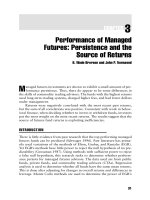
period. Furthermore, the one-day maxima are quite large, ranging from
about 10 to 54 percent for gross volume and 7 to 54 percent for net volume.
Figure 8.1 provides a graphical representation of the “spiky” nature of
MMA trading for the natural gas market. To summarize, although MMAs
tend to focus trading in terms of numbers of contracts in the most liquid
markets, their trading still may represent a large proportion of total market
volume, especially for less liquid futures markets.
The Effect of Large Hedge Fund and CTA Trading on Futures Market Volatility 159
4
The averages reported in Table 8.3 are roughly consistent with results found in
Ederington and Lee (2002) for heating oil futures. Over the June 1993–March 1997
period, they report that the daily trading volume of commodity pools (which include
hedge funds) and commodity trading advisors averages 11.3 percent.
Proportion of Trading Volume
0.5
0.6
0.4
0.3

0.2
0.1
0
4/4/94
4/19/94
5/5/94
5/20/94
6/7/94
6/22/94
7/8/94
7/25/94
8/9/94
8/24/94
9/9/94
9/26/94
FIGURE 8.1 Large Managed Money Account Net Trading Volume as a
Proportion of Total Nearby Trading Volume, Natural Gas Futures Market,
April 4, 1994–October 6, 1994.
c08_gregoriou.qxd 7/27/04 11:13 AM Page 159
To better understand the timing of trading by MMAs relative to trad-
ing by the rest of the market, simple correlation coefficients are computed
between the contemporaneous trading volume of MMAs and the rest of the
market. As reported in Table 8.4, estimated correlation coefficients are all
positive and range from about 0.01 to 0.70. The average correlation across
all markets is 0.39 and 0.38 on a gross and net basis, respectively. Statisti-
cally significant correlations (at the 5 percent level) are observed in 10 mar-
kets for gross volume of MMAs and 10 markets for net volume. The
overwhelmingly positive relationships suggest that MMAs generally trade
when others are trading. This result is the opposite of the negative rela-
tionships that Kodres (1994) found between position changes of hedge

funds and other types of large traders. It is uncertain whether the positive
relationships indicate the potential for stabilizing or destabilizing prices. On
one hand, the positive relationships indicate MMAs tend to trade in more
liquid market conditions, all else being equal. On the other hand, the posi-
tive relationships also may indicate that other traders follow the “leader-
ship” of MMAs, which could destabilize prices through a herd effect
(Kodres, 1994).
160 RISK AND MANAGED FUTURES INVESTING
TABLE 8.4 Correlation between Large Managed Money Account Trading and All
Other Market Trading Volume in 13 Futures Markets, April 4, 1994–October 6, 1994
Correlation Coefficient
Gross Trading Volume of Net Trading Volume of
Futures Market Managed Money Accounts Managed Money Accounts
Coffee 0.35
*
0.33
*
Copper 0.53
*
0.50
*
Corn 0.61
*
0.58
*
Cotton 0.66
*
0.64
*
Crude oil 0.16 0.21

*
Deutsche mark 0.42
*
0.44
*
Eurodollar 0.44
*
0.34
Gold 0.66
*
0.67
*
Live hogs 0.05 0.01
Natural gas 0.07 0.06
S&P 500 0.28
*
0.25
*
Soybeans 0.52
*
0.56
*
Treasury bonds 0.30
*
0.31
*
Note: Managed money accounts are defined as large hedge funds and CTAs. Gross
volume equals long plus short volume. Net volume in this case equals the absolute
value of long minus short volume.
*Statistically significant at the 5 percent level.

c08_gregoriou.qxd 7/27/04 11:13 AM Page 160
Overall, the picture of MMA trading behavior that emerges is mixed.
MMAs tend to focus trading in terms of numbers of contracts in the most
liquid futures markets. However, MMA trading can represent a large pro-
portion of total market volume, especially on certain days and in less liquid
futures markets. Consequently, direct tests are needed to better understand
the market impact of MMA trading. The next section investigates the
relationship between the trading volume of MMAs and price volatility in
futures markets.
Volume and Price Volatility Relationship
Karpoff (1987) provides an extensive and widely cited survey of the method-
ology and results of studies focusing on the relationship between volume and
volatility. The chief difference between model specifications, up to the date
of Karpoff’s survey and since then, is the procedure used to accommodate
persistence in volume and volatility. Due to the lack of a commonly accepted
model specification for the relationship between volume and volatility, three
basic specifications are used in the analysis for this study.
1. Following Chang, Pinegar, and Schachter (1997), the volume and
volatility relationship is modeled without including past volatility.
2. Following Irwin and Yoshimaru (1999), volatility lags are included as
independent variables to account for the time series persistence of
volatility.
3. Following Bessembinder and Seguin (1993), the persistence in volume
and volatility is modeled through specification of an iterative process.
5
Since estimation results for the different model specifications are quite sim-
ilar, only results for a modified version of Chang, Pinegar, and Schachter’s
specification are reported here.
6
Chang, Pinegar, and Schachter (1997) regress futures price volatility on

volume associated with large speculators (as provided by the CFTC large
trader reports) and all other market volume. Including two additional sets
The Effect of Large Hedge Fund and CTA Trading on Futures Market Volatility 161
5
Another approach would be to use a model with a mean equation and a volatility
equation that has both volume and GARCH (generalized autoregressive conditional
heteroskedasticity) terms. This approach is not used due to the limited time series of
observations available for each market. Monte Carlo simulation results generated
recently by Hwang and Pereira (2003) indicate that at least 500 observations are
needed to efficiently estimate models with GARCH effects, substantially more than
the number of daily observations available in this study (130).
6
The full set of regression results can be found in Holt (1999).
c08_gregoriou.qxd 7/27/04 11:13 AM Page 161
of independent variables expands this basic specification. Daily effects on
volatility are well documented, implying that a set of daily dummy variables
should be included. In addition, the estimated specification includes the
open interest for each market. As outlined by Bessembinder and Seguin
(1993), open interest serves as a proxy for market depth, which is antici-
pated to have a negative relationship to volatility. This relationship implies
that changes in volume have a smaller effect on volatility in a more liquid
market (represented by higher open interest). Therefore, the regression
model specification for a given futures market is
s
t
= b
1
+ b
2
MMATV

t
+ b
3
MMAOI
t
+ b
4
AOTV
t
+ b
5
AOOI
t
+
b
6
Mon
t
+ b
7
Tue
t
+ b
8
Wed
t
+ b
9
Thu
t

+ e
t
(8.1)
where s
t
= daily volatility (standard deviation) of futures returns
MMATV
t
= absolute value of net MMA trading volume
MMAOI
t
= absolute value of net MMA open interest
AOTV
t
= other market trading volume
AOOI
t
= other open interest
Mon
t
, Tue
t
, Wed
t
, and Thu
t
= dummy variables that represent
day-of-the-week effects
e
t

= a standard normal error term.
Following Chang, Pinegar, and Schachter (1997) and Irwin and Yoshi-
maru (1999), the extreme-value estimator developed by Parkinson (1980) is
used to estimate daily volatility of futures returns. For a given commodity,
Parkinson’s estimator can be expressed as
s
ˆ
t
= 0.601 ln(H
t
/ L
t
) (8.2)
where H
t
= trading day’s high price
L
t
= the day’s low.
Wiggins (1991) reports that extreme-value estimators are more efficient
than close-to-close estimators in many applications. Previous empirical
results suggest that a positive relationship is expected between volume and
volatility. They also suggest a negative relationship between volatility and
open interest, as shown by Bessembinder and Seguin (1993) for example.
However, open interest within any six-month period may not vary enough
to efficiently estimate its impact on volatility. For the same reason, it is pos-
sible that daily dummy variables will not exhibit the U-shape documented
in previous volatility studies.
162 RISK AND MANAGED FUTURES INVESTING
c08_gregoriou.qxd 7/27/04 11:13 AM Page 162

Table 8.5 reports the estimated coefficients, corresponding t-statistics,
and adjusted R
2
for each market. Due to the relative insignificance of the
day-of-the-week variables, only the F-statistic for testing the joint significance
of the dummy variables is reported. As shown by this F-statistic, significant daily
The Effect of Large Hedge Fund and CTA Trading on Futures Market Volatility 163
TABLE 8.5 Volatility Regression Results for 13 Futures Markets, April 4,
1994–October 6, 1994
MMA Rest of F-Statistic
MMA Rest of Net Nearby for
Futures Net Nearby Open Open Daily Adj.
Market Intercept Volume Volume Interest Interest Effects R
2
Coffee 3440.1
*
−0.1200 0.4590
*
−0.1444
*
−0.1831
*
1.31 0.51
(6.39) (−0.73) (11.19) (−4.85) (−6.31)
Copper 522.6
*
0.0973
*
0.1091
*

−0.0018 −0.0214
*
1.12 0.61
(3.98) (3.22) (9.67) (−0.37) (−4.53)
Corn 916.5
*
0.0411
*
0.0253
*
−0.0147
*
−0.0046
*
1.15 0.49
(3.17) (2.30) (6.41) (−3.53) (−1.98)
Cotton 331.7 0.0379 0.1279
*
0.0070 −0.0009 0.97 0.41
(1.57) (0.98) (6.77) (0.71) (−0.14)
Crude oil 739.4
*
0.0539
*
0.0357
*
−0.0189
*
−0.0094
*

1.85 0.44
(2.69) (2.24) (9.05) (−4.22) (−3.38)
Deutsche 184.5 0.0088 0.0121
*
0.0019 −0.0019 4.06
*
0.45
mark (1.64) (1.09) (7.94) (1.01) (−1.57)
Eurodollar 35.7 0.0010
*
0.0004
*
−0.0002
*
−0.0001 0.38 0.69
(1.60) (3.69) (11.61) (−3.88) (−0.24)
Gold 74.7 0.0234
*
0.0154
*
−0.0010 −0.0003 2.07 0.63
(0.71) (3.60) (7.97) (−0.77) (−0.29)
Live 290.0 0.3929
*
0.2272
*
0.0081 −0.0306
*
1.10 0.30
hogs (1.04) (3.55) (5.74) (0.29) (−3.05)

Natural 120.6 0.1115
*
0.1399
*
0.0256
*
0.0036 0.52 0.47
gas (0.42) (2.76) (8.94) (2.51) (0.26)
S&P −657.7
*
0.0268
*
0.0099
*
−0.0008 0.0035
*
1.03 0.53
500 (−3.61) (3.34) (10.19) (−0.45) (3.79)
Soybeans −121.2 0.0140 0.0423
*
−0.0132 −0.0003 1.05 0.57
(−0.44) (0.71) (9.94) (−1.61) (−0.09)
Treasury 83.8 0.0126
*
0.0018
*
−0.0006 −0.0006 2.16 0.69
bonds (0.78) (4.75) (12.96) (−0.39) (−1.93)
MMA = managed money accounts, which are defined as large hedge funds and CTAs.
The figures in parentheses are t-statistics. The F-statistic tests the null hypothesis

that parameters for the day-of-the-week dummy variables jointly equal zero.
*Statistically significant at the 5 percent level.
c08_gregoriou.qxd 7/27/04 11:13 AM Page 163
effects are observed only for the deutsche mark futures market. The average
adjusted R
2
across all 13 markets is 0.52, indicating a reasonable fit of the
models, particularly in light of the relatively small sample size. The estimated
coefficient for MMA trading volume is significantly positive at the 5 percent
level in nine markets, with the remaining four markets having insignificant
coefficients (coffee, cotton, deutsche mark, and soybeans). All of the esti-
mated coefficients for the rest of market volume are significant and positive
at the 5 percent level. Therefore, as expected, a positive relationship is exhib-
ited between trading volume and price variability, regardless of the trader
type (MMA or all other). Four of the estimated coefficients for MMA open
interest are significantly negative (coffee, corn, crude oil, and eurodollar),
while one is significantly positive (natural gas). For the rest of market open
interest, coefficients are negative and significant in five markets (coffee, cop-
per, corn, crude oil, and hogs) and significantly positive in one market (S&P
500). As mentioned previously, the mixed results for open interest are not
surprising due to the relatively short time period studied.
Previous studies (e.g., Chang, Pinegar, and Schachter 1997) estimate
volatility effects of different trader types by comparing the relative size of
the parameter estimates associated with the traders. For example, estimates
of b
2
and b
4
from regression equation 8.1 could be compared to determine
the volatility effects of MMAs and all other traders. However, this com-

parison can be misleading if the means of the respective independent vari-
ables are not of similar magnitudes. A better approach is to compare
volatility elasticities evaluated at the means of the independent variables.
Estimates for the volatility elasticity of volume and open interest are
reported in Table 8.6. The volatility elasticity of MMA volume ranges from
−0.02 to 0.14, with a cross-sectional average of 0.09. This implies, on aver-
age, that a 1 percent increase in MMA trading volume leads to about a one-
tenth of 1 percent increase in futures price volatility. The volatility elasticity
of all other volume ranges from 0.54 to 1.19, with an overall average of
0.86. This estimate means that a 1 percent increase in all other market vol-
ume (besides MMA volume) leads to slightly less than a 1 percent increase
in futures price volatility. Therefore, on a percentage basis, increases in
MMA trading volume lead to much smaller increases in volatility than do
increases in all other market volume. Finally, it is interesting to note that
open interest elasticities for MMAs average −0.10, indicating that MMA
trading contributes positively to market depth and liquidity.
Explaining the Volume and Volatility Relationship
The results presented in the previous section provide strong evidence of a
positive relationship between MMA trading volume and futures price
164 RISK AND MANAGED FUTURES INVESTING
c08_gregoriou.qxd 7/27/04 11:13 AM Page 164
volatility. However, on its own, this result is not sufficient to conclude that
MMA trading is beneficial or harmful to economic welfare. A positive rela-
tionship between MMA trading volume and market volatility is consistent
with either a private information hypothesis (e.g., Clark 1973), where the
information-driven trading of MMAs tends to move prices closer to
equilibrium values, or a noise trader hypothesis (e.g., De Long, Schleifer,
Summers, and Waldman 1990), where MMA trading is based on “noise” such
as trend-chasing or market sentiment and tends to move prices further from
equilibrium values. Weiner (2002, p. 395) states the issue in succinct terms:

. . . the concern over whether these funds have a positive or negative
effect on market functioning comes down to whether the funds can be
characterized as “smart money”—undertaking extensive analysis on
possible changes in future industry, macroeconomic, political, and so
forth conditions and their likely consequences for prices—or “dumb
money”—noise traders chasing trends or herding sheep, buying and
selling because others are doing so.
Following French and Roll (1986), three tests are used in this study in an
attempt to distinguish between these two hypotheses.
The Effect of Large Hedge Fund and CTA Trading on Futures Market Volatility 165
TABLE 8.6 Estimates of the Volatility Elasticity of Volume and Open Interest
for 13 Futures Markets, April 4, 1994–October 6, 1994.
Rest of Rest of
Futures MMA Net Nearby MMA Net Nearby
Market Volume Volume Open Interest Open Interest
Coffee −0.02 1.33 −0.43 −1.17
Copper 0.08 0.76 −0.02 −0.40
Corn 0.08 0.63 −0.22 −0.55
Cotton 0.03 0.60 0.06 −0.02
Crude oil 0.08 1.19 −0.26 −0.49
Deutsche mark 0.04 1.05 0.07 −0.31
Eurodollar 0.13 0.98 −0.59 −0.06
Gold 0.12 0.82 −0.04 −0.04
Live hogs 0.10 0.54 0.07 −0.11
Natural gas 0.08 0.69 0.15 0.03
S&P 500 0.11 1.22 −0.07 1.00
Soybeans 0.03 1.19 −0.12 −0.02
Treasury bonds 0.14 1.11 −0.01 −0.33
MMA = managed money accounts, which are defined as large hedge funds and CTAs.
c08_gregoriou.qxd 7/27/04 11:13 AM Page 165

Variance Ratio Tests Under market efficiency, price changes follow a ran-
dom walk. Therefore, return variance for a long holding period is equal
to the sum of the daily return variances. However, under the noise trader
hypothesis, the cumulated daily return variances are expected to be greater
than the long holding period variance. This assumes that, over a longer
holding period, the market corrects errors associated with noise trading.
The daily variances include the effects of noise trading, while the longer
holding period variance presumably does not. Therefore, the presence of
noise trading can be identified through an analysis of return variance ratios
over different holding periods.
Variance ratios are computed following the methodology of Campbell,
Lo, and MacKinlay (1997). The q-day variance ratio is
(8.3)
where s
2
q
= q-day holding period return variance
s
2
1
= daily holding period return variance.
Note that overlapping q-period returns are used to estimate s
2
q
and one-day
returns are used to estimate s
2
1
. The use of overlapping returns increases
the efficiency of the variance ratio estimator.

7
For a given commodity, the
standardized test statistic to test the null hypothesis that the variance ratio
equals 1 is
(8.4)
where nq + 1 = number of original daily price observations.
Campbell, Lo, and MacKinlay (1997) show that y
q
approximately follows
a standard normal distribution in large samples. Variance ratios and asso-
ciated test statistics are computed for six different holding periods: for q =
2, 3, 5, 10, 15, and 20 days.
ψ
qq
nq VR
qq
q
=−
−−






−
()
()()
/
1

22 1 1
3
12
VR
q
q
q
=
⋅
σ
σ
2
1
2
166 RISK AND MANAGED FUTURES INVESTING
7
The formulas for the variance estimators are found on pp. 52–53 in Campbell, Lo,
and MacKinlay (1997). One technical issue is how to handle the computation of
futures returns when nearby futures price series roll from the “old” nearby contract
to the “new” nearby contract. To resolve this issue, returns for the first active day
of the “new” nearby contract are computed using the previous day’s price for the
“new” contract, rather than the previous day’s price from the “old” contract.
c08_gregoriou.qxd 7/27/04 11:13 AM Page 166
An important statistical issue arises when interpreting the variance
ratio test results. Specifically, what constitutes evidence against the null
hypothesis? If variance ratios across holding periods are independent, then
rejection of the null hypothesis of unity for one holding period is sufficient
to reject the joint null hypothesis that variance ratios equal unity across all
holding periods. Because of overlapping holding periods, it is unlikely that
the independence assumption is valid. As a result, individual hypothesis

tests likely have a higher probability of Type I error than the specified sig-
nificance level.
To assess the joint significance of variance ratios correctly across hold-
ing periods, a joint test statistic is needed. The Bonferroni inequality pro-
vides a simple means for testing the joint null hypothesis that test statistics
are not different from unity. The inequality provides an upper bound for
rejection of the joint null hypothesis when the test statistics are correlated.
Intuitively, the Bonferroni test simple scales up the p-value of the most sig-
nificant test statistic to account for the dependency. Miller (1966) provides
a full explanation of the Bonferroni inequality and resulting joint testing
procedure.
To implement the Bonferroni joint test for a given commodity, we
define the maximum standardized test statistic as
(8.5)
where y
q
= standardized test statistic for the q-day holding period.
The joint null hypothesis is rejected at the significance level a if y
max
is
greater than the critical value defined by
(8.6)
where f(
.
) = standard normal cumulative distribution function
c = number of restrictions tested
Because variance ratios are estimated for six holding periods, a joint
hypothesis test for a given futures market imposes six restrictions. As a
result, the critical value for the Bonferroni joint test at the 5 percent level
is 2.63.

1
2
−=
φ(ψ)
α
/c
ψψ
max
max=
{}
q
q
The Effect of Large Hedge Fund and CTA Trading on Futures Market Volatility 167
c08_gregoriou.qxd 7/27/04 11:13 AM Page 167
Table 8.7 presents variance ratios and standardized test statistics for
each of the 13 markets. In only 2 variance ratios out of 78 is the null
hypothesis of unity rejected. The two significant ratios suggest the possibil-
ity of a short-run noise trading component in the gold market. The signifi-
cant negative test statistics for the two-day and three-day holding periods
indicate that two- and three-day holding period return variances are less
than two and three times the estimated daily variance. This fact implies the
daily return variances are larger due to the noise component. However, this
noise component is traded away in the long run, as shown by the insignifi-
cant test statistics for the longer holding periods. The gold market also is
the only market out of 13 where the Bonferroni joint test statistic is signif-
icant. This rejection rate (0.077) is only slightly greater than would be
expected based on random chance and a 5 percent significance level. Over-
all, the variance ratio tests for this sample period do not support the noise
trader hypothesis, but instead support the private information hypothesis
for MMA trading.

Because the sample period considered in the previous tests is somewhat
limited, a reasonable question is whether the results are sensitive to differ-
ent time periods and longer sample periods. The first alternative sample
period considered is the previous six-month period from October 1, 1993,
through March 31, 1994. As shown in Table 8.8, only 6 of 78 variance
ratios are significantly different from unity for this sample period. The Bon-
ferroni joint test statistic is significant only for the eurodollar futures mar-
ket, which again is only slightly greater than what would be expected based
on random chance. The second alternative sample period considered is sub-
stantially longer and includes the previous six-and-one-quarter-year period
from January 4, 1988, through March 31, 1994. As shown in Table 8.9,
only 17 out of 78 variance ratios are significantly different from unity.
However, the Bonferroni joint test statistic is significant for 4 of the 13 mar-
kets (cotton, crude oil, Eurodollar, and S&P 500), more than would be
expected based on random chance.
The last finding indicates that variance ratio test results may be sensi-
tive to the use of a relatively small sample size. Nonetheless, the variance
ratio results for alternative sample periods do not provide convincing evi-
dence that the conclusion reached on the basis of the original sample period
is invalid. That is, variance ratio tests do not indicate substantial deviations
from market efficiency that would be associated with noise trading on the
part of MMAs. Instead, the results are more consistent with the hypothesis
that MMAs base their trading on valuable private information.
Positive Feedback Trading Tests Buying after price increases and selling
after price declines characterizes positive feedback trading. The existence of
168 RISK AND MANAGED FUTURES INVESTING
c08_gregoriou.qxd 7/27/04 11:13 AM Page 168
The Effect of Large Hedge Fund and CTA Trading on Futures Market Volatility 169
TABLE 8.7 Variance Ratio Test Results for 13 Futures Markets, April 4,
1994–October 6, 1994

Holding Period Lengths
Bonferroni
Futures Joint Test
Market 2 Day 3 Day 5 Day 10 Day 15 Day 20 Day Statistic
Coffee 1.08 1.12 1.19 1.25 1.49 1.53 1.21
(0.86) (0.95) (1.00) (0.84) (1.32) (1.21)
Copper 0.92 0.91 0.92 0.96 0.97 1.00 0.86
(−0.86) (−0.69) (−0.42) (−0.15) (−0.07) (0.00)
Corn 0.97 1.07 0.96 0.78 0.98 1.00 0.72
(−0.30) (0.56) (−0.19) (−0.72) (−0.06) (0.01)
Cotton 1.08 1.06 1.10 0.99 0.98 0.86 0.91
(0.91) (0.45) (0.52) (−0.03) (−0.06) (−0.32)
Crude oil 1.09 1.09 1.02 1.26 1.35 1.58 1.33
(1.00) (0.68) (0.11) (0.89) (0.93) (1.33)
Deutsche 1.02 1.04 1.09 1.01 0.78 0.73 0.61
mark (0.17) (0.30) (0.49) (0.04) (−0.60) (−0.61)
Eurodollar 1.12 1.19 1.16 0.78 0.74 0.71 1.43
(1.39) (1.43) (0.81) (−0.75) (−0.69) (−0.67)
Gold 0.71
*
0.72
*
0.70 0.75 0.65 0.61 3.25
*
(−3.25) (−2.16) (−1.58) (−0.86) (−0.94) (−0.90)
Live hogs 1.03 0.97 0.90 0.84 0.74 0.51 1.11
0.35) (−0.21) (−0.54) (−0.54) (−0.69) (−1.11)
Natural gas 0.97 1.06 1.24 1.24 1.18 1.19 1.24
(−0.29) (0.44) (1.24) (0.81) (0.49) (0.43)
Soybeans 1.03 1.09 0.96 0.82 0.99 0.98 0.69

(0.31) (0.69) (−0.23) (−0.59) (−0.02) (−0.03)
S&P 500 0.84 0.93 0.86 0.74 0.75 0.73 1.86
(−1.86) (−0.52) (−0.71) (−0.87) (−0.66) (−0.61)
Treasury 0.88 0.86 0.77 0.52 0.49 0.48 1.63
bonds (−1.35) (−1.06) (−1.18) (−1.63) (−1.37) (−1.19)
The figures in parentheses are Z–statistics.
*Statistically significant at the 5 percent level.
c08_gregoriou.qxd 7/27/04 11:13 AM Page 169
170 RISK AND MANAGED FUTURES INVESTING
TABLE 8.8 Variance Ratio Test Results for 13 Futures Markets, October 1,
1993–March 31, 1994
Holding Period Lengths
Bonferroni
Futures Joint Test
Market 2 Day 3 Day 5 Day 10 Day 15 Day 20 Day Statistic
Coffee 0.78
*
0.74 0.62 0.46 0.44 0.39 2.46
(−2.46) (−1.95) (−1.94) (−1.79) (−1.49) (−1.39)
Copper 0.95 0.98 1.01 1.00 1.02 0.95 0.57
(−0.57) (−0.14) (−0.05) (−0.01) (−0.04) (−0.12)
Corn 1.03 0.97 0.92 1.05 1.31 1.74 1.68
(0.39) (−0.25) (−0.41) (0.16) (0.83) (1.68)
Cotton 1.07 1.09 1.14 1.45 1.65 1.94
*
2.13
(0.76) (0.67) (0.71) (1.49) (1.72) (2.13)
Crude oil 0.99 1.03 1.03 1.11 1.21 1.39 0.88
(−0.11) (0.20) (0.17) (0.36) (0.56) (0.88
Deutsche 0.97 1.03 1.03 0.87 0.93 0.95 0.43

mark (−0.38) (0.20) (0.14) (−0.43) (−0.18) (−0.12)
Eurodollar 1.22
*
1.25 1.43
*
1.85
*
2.41
*
3.02
*
4.58
*
(2.51) (1.91) (2.21) (2.83) (3.74) (4.58)
Gold 0.98 0.95 0.88 0.74 0.73 0.70 0.87
(−0.22) (−0.35) (−0.60) (−0.87) (−0.72) (−0.68)
Live 1.08 1.10 1.08 1.11 1.19 1.47 1.07
hogs (0.86) (0.76) (0.42) (0.38) (0.51) (1.07)
Natural 1.04 1.12 1.13 1.28 1.38 1.67 1.51
gas (0.40) (0.90) (0.67) (0.92) (1.01) (1.51)
Soybeans 1.06 1.00 0.95 1.03 1.02 1.03 0.66
(0.66) (0.02) (−0.27) (0.11) (0.05) (0.08)
S&P 500 0.93 0.96 1.02 0.87 0.76 0.71 0.82
(−0.82) (−0.28) (0.11) (−0.43) (−0.63) (−0.65)
Treasury 1.04 1.02 1.10 1.09 1.24 1.44 0.99
bonds (0.47) (0.15) (0.50) (0.30) (0.64) (0.99)
The figures in parentheses are Z-statistics.
*Statistically significant at the 5 percent level.
c08_gregoriou.qxd 7/27/04 11:13 AM Page 170
The Effect of Large Hedge Fund and CTA Trading on Futures Market Volatility 171

TABLE 8.9 Variance Ratio Test Results for 13 Futures Markets, January 4,
1988–March 31, 1994
Holding Period Lengths
Bonferroni
Futures Joint Test
Market 2 Day 3 Day 5 Day 10 Day 15 Day 20 Day Statistic
Coffee 0.97 0.96 0.99 0.97 0.98 1.01 1.35
(−1.35) (−1.07) (−0.23) (−0.34) (−0.15) (0.10)
Copper 1.03 1.02 1.00 1.02 1.00 0.98 1.22
(1.22) (0.50) (0.01) (0.27) (0.03) (−0.15)
Corn 1.02 0.97 0.91 0.86 0.88 0.89 1.71
(−0.66) (−0.87) (−1.71) (−1.66) (−1.13) (−0.87)
Cotton 1.10
*
1.11
*
1.12
*
1.18
*
1.27
*
1.34
*
3.86
*
(3.86) (3.06) (2.19) (2.07) (2.50) (2.70)
Crude oil 1.02 1.01 0.91 0.76
*
0.77

*
0.81 2.78
*
(0.97) (0.39) (−1.62) (−2.78) (−2.12) (−1.53)
Deutsche 1.03 1.01 0.98 0.96 1.00 1.03 1.22
mark (1.22) (0.29) (−0.41) (−0.44) (0.00) (0.22)
Eurodollar 1.07
*
1.06 1.04 1.10 1.13 1.20 2.96
*
(2.96) (1.64) (0.64) (1.22) (1.21) (1.58)
Gold 0.97 0.95 0.91 0.90 0.92 0.91 1.63
(−1.18) (−1.43) (−1.63) (−1.13) (−0.78) (−0.70)
Live hogs 1.03 0.99 0.97 0.98 0.95 0.94 1.10
(1.10) (−0.14) (−0.51) (−0.26) (−0.43) (−0.49)
Natural gas 1.02 0.99 1.01 1.11 1.24 1.37
*
2.39
(0.76) (−0.19) (0.11) (1.02) (1.82) (2.39)
Soybeans 1.06
*
1.04 1.04 1.01 1.00 0.98 2.20
(2.20) (1.16) (0.64) (0.06) (−0.01) (−0.14)
S&P 500 0.94
*
0.90
*
0.84
*
0.72

*
0.70
*
0.70
*
3.24
*
(−2.21) (−2.58) (−2.90) (−3.24) (−2.81) (−2.38)
Treasury 1.02 1.04 0.99 0.93 0.92 0.93 1.10
bonds (0.92) (1.10) (−0.16) (−0.88) (−0.76) (−53)
The figures in parentheses are Z-statistics.
*Statistically significant at the 5 percent level.
c08_gregoriou.qxd 7/27/04 11:13 AM Page 171
172 RISK AND MANAGED FUTURES INVESTING
this type of trading may lead to decreases in market efficiency by creating
excessive volatility. For instance, when new bullish fundamental informa-
tion is received, and price increases to its new fundamental value through
rational trading, positive feedback traders continue to buy, driving price
past its rational value. Following Kodres (1994) and Irwin and Yoshimaru
(1999), positive feedback trading is identified for a given market by esti-
mating this regression model:
(8.7)
where NETMMATV
t
= net trading volume of MMAs (number of long con-
tracts minus number of short contracts) on day t
∆p
t − i
= continuously compounded futures return on day
t − i

e
t
= standard normal error term.
Based on Irwin and Yoshimaru’s results, five lagged price returns are
included in the model for all markets. Note that NETMMATV
t
takes on
positive values when MMAs are net buyers of contracts, negative values
when MMAs are net sellers, and zero when no volume is recorded. Slope
coefficients in equation 8.7 can be thought of as the sensitivities of MMA
“demand” to past price movements. Positive slope coefficients are evidence
of positive feedback trading by MMAs, whereas negative coefficients are
evidence of negative feedback trading. The net feedback effect is given by
the sum of slope coefficients for each regression. The significance of feed-
back trading is determined by testing whether the sum of the estimated
slope coefficients (for lagged price returns) is greater than zero.
Table 8.10 provides estimation results for equation 8.7. The sum of
slope coefficient estimates is positive in nine markets, close to zero in one
market, and negative in three markets. Of the nine positive sums, t-statis-
tics indicate six are significantly different from zero. Thus, statistically sig-
nificant evidence of positive feedback trading among MMAs is found in
about half of the markets studied. The average adjusted R
2
across all 13
markets is 0.09, ranging from a high of 0.35 (cotton) to a low of −0.02 (cof-
fee). Overall, this provides some evidence of positive feedback trading on
the part of MMAs. However, because positive feedback terms explain only
9 percent of the variation in MMA trading volume, it can be concluded that
MMA trading decisions are influenced only in small part by past price
changes. It is interesting to note the similarity of these results to Irwin and

Yoshimaru’s (1999) results for commodity pool trading volume. They
NETMMATV p
ti
i
ti t
=+ +
=
−
∑
αβ ε
1
1
5
∆
c08_gregoriou.qxd 7/27/04 11:13 AM Page 172
TABLE 8.10 Positive Feedback Regression Results for 13 Futures Markets, Large Managed Money Accounts, April 4,
1994–October 6, 1994.
Daily Price Change Lag
Futures Sum of Adj.
Market t − 1 t − 2 t − 3 t − 4 t − 5 Slopes t-statistic R
2
Coffee −2.8 12.8 1.4 7.3 2.6 21.3 0.98 −0.02
(−0.31) (1.44) (0.15) (0.82) (0.28)
Copper 20.1 214.2
*
38.9 141.1 −24.2 390.1
*
2.23 0.05
(0.27) (2.84) (0.52) (1.87) (−0.31)
Corn 251.7

*
190.5
*
−8.4 −61.6 170.0
*
542.2
*
3.77 0.15
(3.85) (3.12) (−0.14) (−1.01) (2.62)
Cotton 628.7
*
214.8
*
230.7
*
63.8 196.4
*
1,334.4
*
6.83 0.35
(7.03) (2.39) (2.57) (0.71) (2.23)
Crude oil −381.8 712.4 −445.0 2,117.2
*
−29.8 −144.2 −0.91 0.02
(−0.44) (0.82) (−0.52) (2.44) (−0.03)
Deutsche mark −160.9 1,729.7
*
468.3 553.2 77.4 2,667.6 1.76 0.01
(−0.22) (2.38) (0.64) (0.76) (0.11)
Eurodollar −21,276.9 8,063.6 −6,149.2 −25,505.1 −15,490.5 −60,358.1

*
−2.10 0.02
(−1.52) (0.58) (−0.44) (−1.83) (−1.11)
173
c08_gregoriou.qxd 7/27/04 11:13 AM Page 173