Commodity Trading Advisors: Risk, Performance Analysis, and Selection Chapter 17 ppsx

CHAPTER
17
CTAs and
Portfolio Diversification:
A Study through Time
Nicolas Laporte
T
he standard mean/variance framework and the concept of efficient fron-
tiers are one way of assessing the portfolio added value of a hedge fund
strategy such as CTAs. However, even if it provides interesting results, this
framework is a two-dimensional one and it gives a static vision of the
CTAs’ industry. Changes in correlation or volatility over time are ignored.
To provide a more dynamic approach, this chapter presents a three-dimen-
sional framework with time as the third variable. It assesses the evolution
of the CTAs’ diversification abilities in a portfolio environment over the
last decade.
INTRODUCTION
Commodity trading advisors (CTAs) are professional money managers.
They manage the assets of their clients using derivative instruments
(futures, forwards, and options) on commodities and money markets
around the world. As an asset category in the alternative investment indus-
try, they are classified as “managed futures.” CTAs’ strategies range from
systematic models to discretionary approaches, the first one being the most
common. CTAs are, most of the time, considered trend followers.
Even though CTAs have existed for a while, only a few studies have
been published about them. The term “CTAs” appears regularly in publi-
cations but, most of the time, is far from being the main topic. Usually
CTAs are mentioned because of their affiliation to the hedge fund industry.
Looking at the practitioner side, the same conclusion can be made.
307
c17_gregoriou.qxd 7/30/04 1:42 PM Page 307

Although it is true that most of the financial players are familiar with CTAs
(CTAs, in fact, have the reputation of being low/negatively correlated to
any asset family, including hedge funds), most of the time, this interesting
feature is all they know about them.
Based on these findings, it is interesting to propose a study focusing
uniquely on the CTA industry with, as main objective, the definition of their
added value in portfolio allocation. Different statistics and portfolio frame-
works (with two or three dimensions) are then considered. Each brings new
information and helps in understanding the managed futures universe. Note
that the three-dimensional framework used with portfolio allocations is
definitively the “pioneering” part of this study.
The chapter is organized in three parts. The first part compares CTAs
with other assets. Two types of values are computed: plain statistics (static
view of the CTA industry) and rolling statistics (dynamic approach, which
takes into account time evolutions). The second part focuses on portfolio
optimization and efficient frontiers. Its objective is to assess the CTAs’
diversification capacity. As in the first part, CTAs are considered under a
static and a dynamic perspective. The dynamic perspective considers time
evolutions using a three-dimensional representation.
CTAs
CTAs’ Quantitative Description
As for any financial asset, the CTAs’ universe is assessable through indices
compiled by several providers. In theory, these indices should match each
other in terms of volatility and performance since they are constructed on the
same original universe (they are supposed to proxy the same industry). In
practice, it is rarely the case. Indices are constructed using different method-
ologies (each methodology defines rebalancing dates, index component
selections, survivorship bias correction, etc.) and, even more important, dif-
ferent data sources. It generates, most of the time, significant patterns dis-
similarity between them.

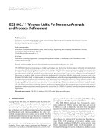
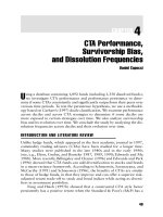
In the case of CTAs, there are two major index providers: CSFB/Tremont
and Barclay Group. It is interesting to consider these two indices
1
(see Fig-
ure 17.1). Because they are traceable from December 1993, our historical
308 PROGRAM EVALUATION, SELECTION, AND RETURNS
1
Of course, the purpose of this comparison is not to run an index quality test. As
mentioned, it is logical to find differences between indices since their methodologies
and universe selection process are different.
c17_gregoriou.qxd 7/30/04 1:42 PM Page 308
index database goes from this date to December 2002, which corresponds
to 109 monthly index levels. From this database, it is easy to extract some
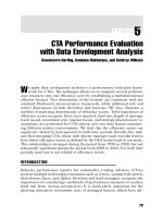
statistics. They are displayed in Figure 17.2 and provide a first step in the
CTAs’ performance assessment.
Clearly, the CTA index and the managed futures index present similar
annualized returns (respectively 6.44 percent and 6.26 percent). However,
their volatilities differ significantly: The annualized standard deviations are,
respectively, 8.39 percent and 11.94 percent (40 percent superior to the Bar-
clay volatility). CSFB/Tremont provides a riskier (or more volatile) view of
the industry than Barclay Group.
In a risk/return framework, CTAs do not have an exceptional profile
compared to other hedge fund investment strategies (e.g., global macro) or
even some traditional equity groups (e.g., real estate investment trust
[REIT] equities).
Actually, only two hedge funds families have lower returns than CTAs:
the dedicated short bias and the emerging markets. Such a finding is not
that surprising, and the origin of their poor results is related to their invest-
CTAs and Portfolio Diversification 309
CSFB/Tremont

Hedge Funds
Indices
Convertible
Barclay
Indices
CSFB/Tremont Hedge
Funds
Barclay CTAs
Arbitrage
Dedicated Short Bias
Emerging Markets
Equity Market Neutral
Event Driven
Fixed Income Arbitrage
Long/Short
The Barclay CTA Index is unweighted and rebalanced at the
beginning of each year. To qualify for inclusion in the CTA
Index, an advisor must have four years of prior performance
history. The restrictions offset high turnover rates of trading
advisors as well as artificially high short-term performance
records.
The Barclay CTA Index also includes six separate subindices
of managed futures programs, based on portfolio composition
and trading style.
For a managed program to be included in any of these sub-
indices, they must have at least 12 full months of prior
performance history, with no extracted performance.
The CSFB/Tremont Hedge Fund Indices are asset
weighted. CSFB/Tremont uses the TASS database.
The CSFB/Tremont universe consists only of funds

with a minimum of US $10 million under management
and a current audited financial statement. Funds are
separated into primary subcategories based on their
investment style. Managed Futures proxies the CTAs’
universe. Funds are not removed from the index until they
are liquidated or fail to meet the financial reporting
requirements. The index is calculated on a monthly basis.
Funds are reselected quarterly.
Discretionary Traders
System Traders
Agricultural Traders
Currency Traders
Diversified Traders
Financial/Metals
Managed Futures
FIGURE 17.1 CSFB/Tremont CTA Index versus Barclay
c17_gregoriou.qxd 7/30/04 1:42 PM Page 309
310 PROGRAM EVALUATION, SELECTION, AND RETURNS
World eq.
Far East eq.
NAREIT
Europe eq.
Europe bds.
North Americas bds.
World bds.
North Americas eq.
CTA Barclay
CSFB Tremont Hedge Fund
CSFB Convertible Arbitrage
CSFB Ded. Short Bias

CSFB Emerging Markets
CSFB Equity Mkt. Ntrl.
CSFB Event Driven
CSFB Fixed Inc. Arb.
CSFB Global Macro
CSFB Long/Short
CSFB Managed Futures
–0.075
–0.050
–0.025
0.000
0.025
0.050
0.075
0.100
0.125
0.150
0.00
0.05 0.10 0.15 0.20
Annualized Return
Annualized Standard Deviation
Annualized
returns
Annualized
std. dev. Min Max
World bonds 0.0581 0.0628 –0.0354 0.0585
North Americas bonds 0.0703 0.0441 –0.0249 0.0384
Europe bonds 0.0682 0.0887 –0.0500 0.0849
World equities
0.0314 0.1503 –0.1445 0.0853

North Americas equities
0.0715 0.1652 –0.1548 0.0938
Europe equities
0.0384 0.1586 0.0037 0.0033
Far East equities
–0.0649 0.1980 –0.1295 0.1676
NAREIT 0.0926 0.1197 0.0075 0.0076
CSFB Tremont Hedge Fund 0.1054 0.0882 0.0096 0.0097
Convertible Arbitrage 0.1013 0.0488 0.0090 0.0090
Ded. Short Bias 0.0079 0.1805 –0.0010 –0.0009
Emerging Markets 0.0489 0.1885 0.0047 0.0042
Equity Mkt. Ntrl.
0.1095 0.0316 0.0092 0.0094
Event Driven
0.1038 0.0643 0.0087 0.0087
Fixed Inc. Arb.
0.0661 0.0416 0.0059 0.0060
Global Macro
0.1396 0.1260 0.0125 0.0127
Long/Short
0.1149 0.1139 0.0105 0.0105
Managed Futures 0.0626 0.1194 0.0045 0.0046
CTA Barclay
0.0644 0.0839 0.0055 0.0057
FIGURE 17.2 Statistics for CTA Performance Assessment
All calculations are based on monthly data from December 1993 to December
2002. Data sources are Morgan Stanley Capital International (equity and bond
indices), NAREIT (REIT index), CSFB/Tremont (hedge fund indices, including the
managed futures index), and Barclay Group (CTA index).
c17_gregoriou.qxd 7/30/04 1:42 PM Page 310

ment styles and their ensuing relation with the markets. Concerning the
dedicated short bias, this strategy lost most of its interest during the strong
telecom/information technology bull period. The emerging markets funds
focus on hazardous businesses; because they invest in debt, equity, and
trade claims of companies located in emerging countries, they deal with an
important lack of transparency and have many uncertainties linked to eco-
nomical, political, and social factors. (The Russian bond default is one
extreme example.)
As with the two previous hedge funds strategies, the relative underper-
formance of CTAs is, in large part, explainable by the specificities of their
business. Future managers focus on a few highly volatile and speculative
markets, which reduces their physical investment opportunities. CTAs did
not really take advantage of the increasing markets globalization (compared
to some other hedge funds families). Moreover, most of them are trend fol-
lowers, meaning that they go long or short with a lag compared to the mar-
kets. In the best cases, this lag reduces their benefits; in the worst cases, it
generates heavy losses. It is true that managers significantly leverage their
positions to increase their returns, but the use of leverage does not com-
pensate for the lack of diversification and the important risk bearing.
Besides these negative issues, investors see in CTAs an interesting
investment vehicle because they have been historically low/negatively cor-
related to the other financial assets. This characteristic is the logic conse-
quence of their business (CTAs do not invest in standard assets but instead
deal with futures, a product not frequently used by the other hedge fund
managers), and it is clearly verified Figure 17.3. CTAs do provide a low
correlation level with standard assets (stocks and bonds) and hedge fund
strategies. Of course, because of the index methodologies differences,
results differ from one index to the other. The values range from −0.207 to
0.376 for the CTA index and from −0.283 to 0.339 for the managed
futures index. The difference in methodologies and data sources between

the two indices is assessed by the managed futures/CTAs index correlation:
The value is 0.805 (a relatively low result for two products proxying the
same industry).
CTAs through Time
Even if findings are interesting and help in defining the CTAs’ behavior rel-
ative to other assets, they give a static view of this investment strategy, so
they are unable to detect any temporal change in return, volatility, or cor-
relation. Time variations are simply ignored.
A dynamic approach that uses rolling windows is therefore warranted.
This technique uses moving subsamples as inputs for the statistics’ compu-
CTAs and Portfolio Diversification 311
c17_gregoriou.qxd 7/30/04 1:42 PM Page 311
CTA
Barclay Futures
CSFB
Hedge
Fund
Conv.
Arb.
Ded.
Short
Bias
Emerging
Markets
Equity
Mkt. Ntrl.
Event
Driven
Fixed
Inc.

Arb.
Global
Macro
Long
Short
CTA Barclay 1
Managed Futures 0.805 1
CSFB Tremont Hedge Fund
0.219 0.073 1
Convertible Arbitrage –0.100 –0.283 0.408 1
Ded. Short Bias 0.213 0.295 –0.471 –0.224
Emerging Markets –0.120 –0.164 0.647 0.349 –0.568 1
Equity Mkt. Ntrl. 0.218 0.158 0.335 0.324 –0.391 0.236 1
Event Driven –0.156 –0.269 0.657 0.598 –0.609 0.699 0.391 1
Fixed Inc. Arb. 0.041 –0.120 0.453 0.546 –0.063 0.299 0.091 0.381 1
Global Macro 0.376 0.239 0.861 0.300 –0.113 0.405 0.207 0.365 0.463 1
Long/Short –0.018 –0.093 0.781 0.267 –0.738 0.591 0.353 0.662 0.205 0.422 1
Europe
Bonds
North
Americas
Bonds
Europe
Equity
North
Americas
Equity
Far East
Equity
NAREIT

NAREIT
Equity
CTA
Barclay Futures
Europe Bonds 1
North Americas Bonds 0.394 1
Europe Equity 0.054 –0.117 1
North Americas Equity –0.189 –0.037 0.781 1
Far East Equity 0.014 –0.109 0.514 0.521 1
0.035 0.005 0.286 0.292 0.089 1
CTA Barclay 0.170 0.366 –0.207 –0.193 –0.094 –0.047 1
Managed Futures 0.310 0.339 –0.197 –0.269 –0.035 –0.093 0.805 1
1
FIGURE 17.3 Correlation of CTAs with Standard Assets and Hedge Fund Strategies
All calculations are based on monthly data from December 1993 to December 2002. Data sources are Morgan
Stanley Capital International (equity and bond indices), NAREIT (REIT index), CSFB/Tremont (hedge fund
indices, including the Managed Futures index) and Barclay Group (CTA index).
312
c17_gregoriou.qxd 7/30/04 1:42 PM Page 312
tation. From the practical perspective, the choice of the subsample length
(or rolling window) is the sensitive step. A large window limits the number
of statistics and smooths results while increasing the econometric signifi-
cance. A small one does exactly the opposite. With a database going from
December 1993 to December 2002, a time period of 36 months is a good
compromise. It allows the generation of 73 sets of statistics (starting in
December 1996).
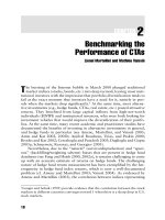
This time approach provides interesting results on the CTAs’ standard
deviation for two reasons (Figure 17.4). First, it highlights the strong insta-
bility of volatility through time, which was not assessable with the previ-
ous statistics (see Figure 17.2). Second, even if the range of values differs

from one index to the other (from 0.067 to 0.092 for the CTA index and
0.099 to 0.131 for the managed futures index), the trend is similar, which
is comforting (the two indices are a proxy of the same universe). Note that
the managed futures standard deviation is more volatile than the CTA
standard deviation. It confirms observations obtained with the previous
statistics.
Another interesting application for the rolling statistics is on correlations.
Based on a 36-month window, the correlation is estimated exactly as for the
standard deviation. The main results are shown in Figures 17.5 and 17.6.
Figure 17.5 illustrates the evolution of the CTAs’ correlation with several
equity indices. Similar to the standard deviation, there is clearly instability
through time, and the two indices have a similar trend. The correlation
had a strong move-down in late summer 1998 and decreased since that
period. In December 2002, CTAs are negatively related to the equity indus-
try. For the CTAs’ index, the values range from −0.59 (North Americas/
CTAs and Portfolio Diversification 313
0.06
0.07
0.08
0.09
0.10
0.11
0.12
0.13
0.14
Dec-96
Jun-97
Dec-97
Jun-98
Dec-98

Jun-99
Dec-99
Jun-00
Dec-00
Jun-01
Dec-01
Jun-02
Dec-02
CTAs' Barclay CSFB/Tremont Managed Futures
FIGURE 17.4 Evolution of CTA Standard Deviation
The standard deviation is annualized and estimated on a 36-month rolling basis.
The database covers the period December 1993 to December 2002 and the first
standard deviation is estimated in December 1996.
c17_gregoriou.qxd 7/30/04 1:42 PM Page 313
CTAs) to −0.21 (REIT/CTAs). This negative correlation implies that CTAs
provide positive returns when equities do not, which is a nice feature.
More generally, when looking at the overall period covered by Figure
17.5, CTAs tend to be positively or neutrally correlated to markets in bull-
ish periods while being negatively correlated in bearish markets.
314 PROGRAM EVALUATION, SELECTION, AND RETURNS
–
0.25
0.00
0.25
0.50
0.75
1.00
Dec-96
Jun-97
Dec-97

Jun-98
Dec-98
Jun-99
Dec-99
Jun-00
Dec-00
Jun-01
Dec-01
Jun-02
Dec-02
CSFB / CTA CSFB / M.Fut M.Fut / CTA
FIGURE 17.6 Correlation at the Two CTA Indices with Each Other and with the
CTA/Tremont Hedge Fund Index
The correlation is estimated on a 36-month rolling basis. The database covers the
period December 1993 to December 2002, and the first correlation is estimated in
December 1996.
–
0.60
–
0.40
–
0.20
0.00
0.20
0.40
0.60
Eur_eq/M_Fut N_Am_eq/M_Fut F_East_eq/M_Fut NAREIT/M_Fut
–
0.60
–

0.40
–
0.20
0.00
0.20
0.40
0.60
Dec-96
Jun-97
Dec-97
Jun-98
Dec-98
Jun-99
Dec-99
Jun-00
Dec-00
Jun-01
Dec-01
Jun-02
Dec-02
FIGURE 17.5 Evolution of CTA Correlation with Equity Indices
The correlation is estimated on a 36-month rolling basis. The database covers the
period December 1993 to December 2002, and the first correlation is estimated in
December 1996.
c17_gregoriou.qxd 7/30/04 1:42 PM Page 314
Figure 17.6 shows the correlation of the two CTAs indices with each
other and the correlation with the Credit Suisse First Boston FBCS/Tremont
Hedge Fund index. The two CTAs versus hedge funds profiles are identi-
cal, but the correlation through time (as for the standard deviation) fluc-
tuates. With the progression of the years, the managed futures indices are

less and less related to the hedge fund industry. In December 2002 (based
on the last 36-month values), the correlation is around zero. With such
results, CTAs also can be expected to be a source of diversification for
hedge fund portfolios.
Note that the correlation between the two CTAs indices ranges from
0.6 at the beginning of 1997 to almost 1 in December 2002. This conver-
gence is consistent with the previously observed common trends on stan-
dard deviation and correlation for the two indices. It reflects increasing
similarities on the different index provider’s universes. (The current data
available for the index computations are definitively more transparent and
accessible for any index provider than they were six or eight years ago.)
CTAs AND PORTFOLIO OPTIMIZATION
Our findings lend support to the claim that CTAs are without a doubt an
extra source of diversification in portfolios. This claim is far from being
new and is actually the main market players’ belief about CTAs. However,
because something everyone believes is not necessarily true, we now focus
on verifying this assumption through a simple portfolio optimization frame-
work. This framework is based on three steps:
1. Creation of different pools of assets, including pools without CTAs.
2. Construction of efficient frontiers with each of the pools.
3. Comparison of the efficient frontiers built with CTAs to those con-
structed without CTAs and determination if this hedge fund strategy
adds value at the portfolio level or not in terms of risk/returns.
Recall that, in a risk/return framework, the efficient frontier represents all
the risk/return combinations where the risk is minimized for a specific
return (or the return is maximized for a specific risk). Each minima (or
maxima) is reached thanks to an optimal asset allocation. The process of
constructing efficient frontiers through an asset weight optimization is sum-
marized in this definition:
For all possible target portfolio returns, find portfolio weights (i.e.,

asset allocation) such as the portfolio volatility is minimized and the
following constraints are respected: no short sale, full investment, and
weight limits if any.
CTAs and Portfolio Diversification 315
c17_gregoriou.qxd 7/30/04 1:42 PM Page 315
Clearly, the resulting efficient frontier depends on the returns, volatil-
ity, and correlations of the considered assets, but it also depends on the con-
straints (maximum and minimum weight limit, no short selling, and full
investment) fixed by the portfolio manager.
Assets used in this chapter are indices only. There are advantages in
considering indices for a portfolio optimization, because they cover market
areas large enough to avoid an excessive number of elements in the pool
and cover the most relevant asset classes. Of course, they must be selected
in such a way they do not overlap each other. Practically, the chosen assets
are either standard indices (equities and bonds) or alternative investment
indices (hedge funds):
■ Bonds indices: MSCI North Americas, MSCI Europe.
■ Stock indices: MSCI North Americas, MSCI Europe, MSCI Far East,
NAREIT index.
■ Hedge funds indices: CSFB/Tremont and its nine subindices (Con-
vertible Arbitrage, Dedicated Short Bias, Emerging Markets, Equity
Market Neutral, Event Driven, Fixed Income Arbitrage, Global Macro,
Long/Short, Managed Futures).
■ Two CTAs indices are available. To avoid the multiplication of figures,
only the managed futures index from CSFB/Tremont is considered for
the portfolio optimizations.
Based on a database of 108 monthly returns (December 1993 to
December 2002), four pools of indices are created (see Figure 17.7). The
first one contains only traditional assets (stocks and bonds). The second
corresponds to the first one plus CTAs. The third one has traditional assets

and all the hedge funds strategies except CTAs. Finally, the last one is made
of all traditional assets and hedge funds strategies including CTAs. Whether
to consider or not consider CTAs in the pools should affect the generated
efficient frontiers and highlight any diversification capacity of CTAs.
Concerning the portfolio optimizations, two frameworks are used: a
classical two-dimensional risk-return framework and a three-dimensional
one (a risk/return/time framework; the time being introduced with rolling
statistics). The three-dimensional framework should capture time changes,
which are rarely presented in portfolio allocation studies.
Portfolio Optimization and Constraints
Before being specific about CTAs, it is important to have a brief reminder
of portfolio optimization and constraints. As mentioned, the efficient fron-
tier’s shape strongly depends on the weight threshold applied during the
316 PROGRAM EVALUATION, SELECTION, AND RETURNS
c17_gregoriou.qxd 7/30/04 1:42 PM Page 316
portfolio optimization. The “best” efficient frontiers always are built when
t
here are no weight limits (see Figures 17.8a and b.) However, unconstrained
efficient frontiers do not represent real investment conditions. Most of the
time, a “free” optimization allocates unrealistic weights to the assets. They
also do not fit, most of the time, either the investor’s legal requirements
and/or the risk profile (see Figure 17.9).
CTAs’ Portfolio Optimization, Full Data
This section determines whether the common belief about CTAs, that CTAs
are an attractive investment vehicle and they bring diversification to port-
folios, is true. We have seen that, from the statistical point of view, there is
a high probability of CTAs adding value to portfolios. But, do they really
add value for all types of portfolios, or only under a particular asset allo-
cation environment? To answer to these questions, several efficient frontiers
are generated with various baskets of assets and constraints.

Varying the asset to be included in portfolios and the constraints high-
lights several interesting features about CTAs. In a traditional asset uni-
verse (no hedge funds), CTAs do in fact add value to conservative
CTAs and Portfolio Diversification 317
Convertible
Arbitrage
Dedicated Short Bias
Emerging Markets
Equity Market Neutral
Event Driven
Fixed Income Arbitrage
Long/Short
Managed Futures
Europe bonds
Europe equity
North American bonds
North American equity
Far East equity
REIT equity
Pool of assets I x x
x
x
x
x
x
x
x x
x x x
x
x

x
x
x
x
x
x x
x
x
x
x
x x
x x
x
x
x x
x x
x
x
x x
x x
Hedge Funds Indices
Pool of assets II
Pool of assets III
Pool of assets IV
FIGURE 17.7 Four Pools of Indices
Each pool is made of several assets: equity indices (MSCI), bond indices (MSCI),
a REIT index (NAREIT), different hedge funds strategies (CSFB/Tremont), and a
CTA index (Barclay Group).
c17_gregoriou.qxd 7/30/04 1:42 PM Page 317
portfolios (they significantly increase low-risk portfolio returns). But this

return enhancement rapidly decreases and becomes null when considering
higher risk portfolios (see Figures 17.10 and 17.11a). The return enhance-
ment is verified in constrained and unconstrained environments. With a
constant asset universe, the lower the weight threshold is, the more impor-
tant is the CTAs’ added value, which was expected (assets such as hedge
funds are rapidly capped).
Finally, when considering a portfolio mixing traditional and alternative
assets, CTAs also add value but only if the optimization process is con-
strained (see Figures 17.10 and 17.11b). The added value itself is much
smaller than when constructing efficient frontiers with standard indices.
CTAs apparently cannot compete with the other hedge funds strategies on
a free asset allocation construction. Once again, this conclusion was
expected. In fact, even if CTAs are low correlated with the hedge funds
industry, their returns are not exceptionally impressive. And correlation is
only one of the factors to be considered in a portfolio optimization. Weight
constraints, returns, and volatility (standard deviation) definitely influence
the definition of the optimal weight of an optimal portfolio.
318 PROGRAM EVALUATION, SELECTION, AND RETURNS
0.03 0.04 0.05 0.06 0.07 0.08 0.09
0.065
0.070
0.075
0.080
0.085
0.090
0.095
0.100
0.105
0.110
Risk (annualized standard deviation)

Return (annualized)
0 0.02 0.04 0.06 0.08 0.1 0.12 0.14
0.08
0.09
0.10
0.11
0.12
0.13
0.14
0.15
Risk (annualized standard deviation)
Return (annualized)
AB
FIGURE 17.8 Efficient Frontiers and Asset Allocation Constraints
Two efficient frontiers are built on the pool of assets II (Figure A). The two optimi-
zations assume a full investment and no short sale. The first efficient frontier (solid
line) is generated without weight constraints and the second one (dashed line) with
weight constraints (a maximum 50 percent allocation per asset). If the weight
increases (the constraint is less strict), the efficient frontier tends to be similar to
the unconstrained efficient frontier (Figure B, dashed line). Four efficient fron-
tiers (solid lines) are built on the pool of assets IV (portfolio fully invested and no
short sale).
c17_gregoriou.qxd 7/30/04 1:42 PM Page 318
As an example, let us focus on one portfolio optimization (Figures
17.11a and b). These assumptions are applied on the pool of assets IV (15
members): no constraints, full investment, and no short sell. The optimiza-
tion includes assets having the best risk/return profiles. Hedge funds strate-
gies like global macro or the REIT equities are immediately selected, which
is not the case for CTAs. CTAs are not included in any efficient portfolio
construction. The asset allocation is totally different when weight restric-

tions are applied: The best risk/return assets are rapidly capped, and the
optimization process considers other assets such as CTAs.
Note that in the real world, portfolio allocations are weight-capped.
No investor takes the risk to be fully invested in a single asset family
(absence of diversification). Moreover, most of the time, investors have to
deal with regulations that forbid excessive weights. As it has been demon-
strated that, in a constrained universe, CTAs add diversification to portfo-
lios (especially when the original portfolio is made of standard assets) this
strategy is worth being considered. It confirms the results discussed earlier
and also investors’ belief about CTAs as a diversification vehicle.
CTAs and Portfolio Diversification 319
1.0
0.75
0.50
0.25
0
0.02
0.04
0.06
0.08
0.10
0.12
0.11
0.10
0.09
0.08
0.07
0.06
Return
Constraint (percent

weight allocation)
Risk
FIGURE 17.9 Consequence of Weight Constraints on the Efficient Surface
The efficient surface is built on the pool of assets II. Leverage is not allowed and
the portfolio is fully invested. For each efficient frontier, the same asset is
constrained (the North Americas index) with an increasing fixed weight in the
portfolio. The range of weight goes from 0 percent (unconstrained portfolio) to
100 percent (portfolio made of a single asset). As a constraint increases, the effi-
cient surface is reduced and tends to a single risk/return combination (100 percent
allocation in a single asset).
c17_gregoriou.qxd 7/30/04 1:42 PM Page 319
320 PROGRAM EVALUATION, SELECTION, AND RETURNS
0.02 0.03 0.04 0.05 0.06 0.07 0.08 0.09
0.075
0.080
0.085
0.090
0.095
0.100
0.105
0.110
Risk (annualized standard deviation)
Return (annualized)
0.04 0.06 0.08 0.1 0.12
0.070
0.075
0.080
0.085
0.090
0.095

Risk (annualized standard deviation)
Return (annualized)
AB
a
b
c
d
FIGURE 17.10 Comparative CTA Portfolio Optimization
In the first figure (A), four efficient frontiers are built with different weight
thresholds (absence of constraints (line a), maximum weight per asset of 0.4 (lines
b), 0.45 (lines c) and 0.5 (lines d)). The assets considered below to the pools I
(standard assets, without CTAs (dashed lines)) and II (standard assets, with CTAs
(solid lines)). The optimizations assume a full investment of the portfolio with no
short sell. With a low cap level, the inclusion of CTAs significantly improve the
performance of risk averse investors.
Similar results are obtained with the pool of assets III/IV (standard and alternative
assets, without/with CTAs) for two of the three efficient frontiers (Figure B). The
performance improvement is less significant than the one observed with the first
figure. CTAs are not included in the unconstrained portfolio (single solid line).
0.02 0.04 0.06 0.08 0.10 0.12 0.14
0.08
0.09
0.10
0.11
0.12
0.13
0.14
0.15
Risk (annualized standard deviation)
Return (annualized)

0.02 0.03 0.04 0.05 0.06 0.07 0.08 0.09 0.10 0.11 0.12 0.13
0.065
0.070
0.075
0.080
0.085
0.090
0.095
0.100
Risk (annualized standard deviation)
Return (annualized)
A
B
FIGURE 17.11 Comparative Unconstrained CTA Portfolio Optimization
In figure A, two unconstrained efficient frontiers are generated on the pools of
assets I (without CTAs, dashed line) and II (with CTAs, solid line). Managed
futures add diversification to low-risk portfolios. The inclusion of CTAs on a pool
of assets including standard (equities and bonds) and alternative (hedge funds)
vehicles is useless in an unconstrained environment (Figure B).
c17_gregoriou.qxd 7/30/04 1:42 PM Page 320
CTAs’ Portfolio Optimization, Rolling Window
Because the previous efficient frontiers use the full database, the results give
an interesting but static view of the CTAs’ diversification ability. Further-
more, time is ignored. Over the period December 1993 to December 2002,
many economical, financial, and even political events impacted the markets
and influenced the CTAs’ industry. Consequently, the inclusion of time as a
parameter in an efficient frontier study should provide interesting results.
In practice, this time perspective is included in the efficient frontier con-
struction simply by combining the portfolio optimization with the rolling
windows technique. For each of the rolling windows (subsample of the his-

torical database), an efficient frontier is computed. Each efficient frontier
reflects the subsample allocation structure.
Because this approach considers three different variables, the clearest
way to represent results is to construct a three-dimensional framework, the
axes being the risk, the return, and the time. The resulting surface is gen-
erated based on a sequence of efficient frontiers, and it can be considered
as a three-dimensional efficient surface. Practically, the surface is built in
this way:
■ Select a 36-month data range, starting in December 1993.
■ Compute portfolio statistics for this range of data.
■ Construct the efficient frontier.
■ Move to the next month and start the same process again.
■ Repeat the same procedure for each month until December 2002.
The efficient surface presented in Figure 17.12 is the result of the con-
strained portfolio optimization through time on pool of assets II. The sur-
face is unstable; significant jumps in values and some brutal length
reductions are observable. Nevertheless, this instability is logical. Because
the input needed for each of the efficient frontiers (the rolling statistics) var-
ied significantly through time, so does the resulting efficient surface. This
instability implies that, every month, the available efficient portfolios are dif-
ferent. They evolve from one month to the next. Some risk/return combina-
tions are not reachable anymore (combinations not accessible by any weight
allocation
2
) or no longer efficient. New combinations also may emerge.
CTAs and Portfolio Diversification 321
2
The same portfolio construction rules are kept through time. The introduction of
leverage, for example, would substantially modify the results.
c17_gregoriou.qxd 7/30/04 1:42 PM Page 321

For example, there were no high risk/return portfolios “available” in
the years 1997 and 1998. High risk portfolios were attainable during the
period 1999 to late 2001, but in December 2002, it was not possible to
invest in such portfolios anymore (in other terms, in December 2002, there
were no weight allocations that enabled the creation of a portfolio with a
high risk/return profile).
Aside from the instability of the efficient frontier through time, it is
interesting to note that the lowest risk level for a portfolio based on the
pool of assets II remains relatively stable (but the returns fluctuate).
The concept of efficient surface and its visualization through a three-
dimensional framework is meaningful. It illustrates the importance of time
322 PROGRAM EVALUATION, SELECTION, AND RETURNS
0
Dec 96
Dec 97
Dec 98
Dec 99
Dec 00
Dec 01
Dec 02
0.05
0.10
0.15
0.20
0.25
0.05
0.10
0.15
0.20
0.25

0.30
Dec 02 Dec 01 Dec 00 Dec 99 Dec 98 Dec 97 Dec 96
Dec 02
Dec 01
Dec 00
Dec 99
Dec 98
Dec 97
Dec 96
0.250
0.225
0.200
0.175
0.150
0.125
0.100
0.175
0.050
0.025
0.30
0.25
0.20
0.15
0.10
0.05
0
0.1
0.2
0.3
0.4

Time
Time
Time
Risk
Risk
Return
Return
FIGURE 17.12 Efficient Surface
The efficient surface is built on the pool of assets II with a 30 percent weight
constraints. The efficient surface is an interpolation derived from a sequence of
efficient frontiers (generated on a monthly basis, starting December 1996). The
surfaces highlight the instability of efficient portfolios through time.
c17_gregoriou.qxd 7/30/04 1:42 PM Page 322
variations in portfolio construction. And it explicitly highlights the impor-
tance, for portfolio managers, of considering dynamic allocations.
But there is another way to look at the efficient surface and to extract
information; it consists of comparing two efficient surfaces: one built on a
pool of assets including CTAs and one built on a similar pool without
CTAs. Such an approach determines periods where CTAs did add value to
the portfolios, and at the same time it quantifies the extra returns. This
comparison can be performed easily because the efficient frontiers are built
on the same framework. Note that interpolation is used during the creation
of the efficient surfaces. It is therefore important to choose a sufficiently
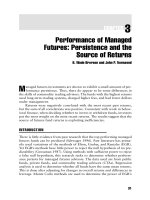
fine partition (or grid) for the range of standard deviations.
Compared to Figure 17.12, the interpretation of the resulting surface is
straightforward and much more explicit in Figure 17.13. When there is no
added value in including CTAs in a portfolio, the surface (a “diversification
surface”) is flat. When it is penalizing to include CTAs (in terms of
risk/return), the surface goes below zero.
3

When CTAs add value to the port-
folio, the surface has a positive shape. The shape itself depends on how much
the asset adds in terms of returns. With this representation, “abnormal”
reliefs can be seen. They appear only if the efficient frontier including CTAs
has a wider range of risk/return combinations than the one without CTAs or
if it is the contrary (the efficient frontier without CTAs has a wider range of
combinations than the one with CTAs). In these cases, peaks (respectively
positive and negative) emerge on the diversification surface; the peaks’
height are equal to the return provided by the considered portfolio.
The diversification surface presented in Figure 17.13 reflects the differ-
ences between the efficient portfolios generated with the pool of assets II
(pool that includes CTAs) and the ones generated with the pool of assets I
(no CTAs in this pool). The constraints are no short selling, full investment,
and a weight threshold (30 percent maximum per asset).
From the diversification surface, one clearly sees that, except for the
period October 1996 to March 1997, managed futures generated new low
risk portfolios (peaks on the surface with a height equal to the new portfo-
lio’s return).
CTAs also occasionally bring diversification to medium-risk portfolios.
It is significant during 1999 and then decreases a lot the first quarter of
2000. Therefore, Figure 17.13 confirms the previous observations on CTAs.
They add value to portfolios, but this diversification ability is not constant
over time and not verified for all efficient portfolios.
CTAs and Portfolio Diversification 323
3
This case was not observable because no minimum weight was imposed.
c17_gregoriou.qxd 7/30/04 1:42 PM Page 323
324 PROGRAM EVALUATION, SELECTION, AND RETURNS
Dec 02
Dec 01

Dec 00
Dec 02
Dec 01
Dec 00
Dec 99
Dec 99
Dec 98
Dec 98
Dec 97
Dec 97
Dec 96
Dec 96
0.08
0.06
0.04
0.02
0.10
0.05
0.05
0.10
0.10
0.15
0.15
0.20
0.20
0.25
0.25
0
0.08
0.07

0.09
0.06
0.05
0.04
0.03
0.02
0.01
0.10
0
Return
Return
Risk
Risk
Time
Time
FIGURE 17.13 Diversification Surface
Diversification surface generated using two efficient surfaces; the first one has some
exposure to CTAs while the second one does not invest in any CTAs. The shape of
the surface highlights the CTAs’ diversification capacity through time and for
different risk levels; the higher the “relief,” the more important the CTAs’ added
value for a portfolio.
c17_gregoriou.qxd 7/30/04 1:42 PM Page 324
CONCLUSION
This chapter confirms that CTAs add value to portfolios but only under cer-
tain conditions. Results demonstrated that CTAs bring diversification as
long as the asset allocation environment is constrained. This diversification
ability clearly increases the lower the weight threshold is (the stricter the
constraints are) and if the included assets are only standard assets.
Aside from the demonstration of the CTAs’ added value, the rolling
window analyses illustrate the time variability of the efficient frontiers. This

finding was expected because the input factors are themselves evolving
through time, proving the necessity of using dynamic asset allocation.
Moreover, the analyses also reveal that CTAs did not systematically
improve portfolio returns over the period 1996 to 2002.
More generally, the three-dimensional graphs presented are one of the
first attempts at using surfaces as a visualization and assessment tool for
asset allocation. The frameworks prove interesting for decision making,
understanding efficient portfolio constructions, and temporal dynamics. It
is exciting to represent simultaneously the evolution of three variables. And
with the growing information technology resources, this graphical repre-
sentation should be used more frequently in the future.
CTAs and Portfolio Diversification 325
c17_gregoriou.qxd 7/30/04 1:42 PM Page 325