Introduction to Modeling and Control of Internal Combustion Engine Systems P2 ppsx

1.5 Structure of the Text 19
In heavy-duty applications, where fuel economy is a top priority, lean de-
NO
x
systems using a selective catalytic reduction (SCR) approach are an
interesting alternative. Such systems can reduce engine-out NO
x
by approxi-
mately one order of magnitude. This permits the engine to be calibrated at the
high-efficiency/low-PM boundary of the trade-off curve (see Fig. 1.11, early
injection angle). The drawback of this approach is, of course, the need for an
additional fluid distribution infrastructure (most likely urea).
While such systems are feasible in heavy-duty applications, for passenger
cars it is generally felt that a solution with Diesel particulate filters (DPF) is
more likely to be successful on a large scale. These filters permit an engine cal-
ibration on the high-PM/low-NO
x
side of the trade-off. Using this approa ch,
engine-out NO
x
emissions are kept within the legislation limits by using high
EGR rates but without any further after-treatment systems.
Radically new approaches, such as cold-flame combustion (see e.g., [190])
or homogeneous-charge compression ignition engines (HCCI, see [187], [188],
[172] for control-oriented discussion) promise further reductions in engine-out
emissions, especially at part-load conditions.
In all of these approaches, feedforward and feedback control systems will
play an important role as an ena bling technology. Moreover, with ever in-
creasing system complexity, model-based approaches will become even more
impo rtant.
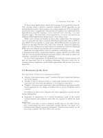
1.5 Structure of the Text

The main body of this text is organized a s follows:
• Chapter 2 introduces mean-value
10
models of the most impo rtant phenom-
ena in IC e ngines.
• Chapter 3 derives discrete-event or crank-angle models for those subsys-
tems that will need such descriptions to be properly controlled.
• Chapter 4 discusses some important control problems by applying a model-
based approach for the design of feedforward as well as feedback control
systems.
In addition to these three chapters, the three appendices contain the fol-
lowing information:
• Appendix A summarizes, in a concise formulation, most of the control
system analysis and sy nthesis ideas that are required to follow the main
text.
10
The term mean-value is used to designate models that do not reflect the en-
gine’s reciprocating and hence crank-angle sampled beh avior, but which use a
continuous-time lumped parameter description. Discrete-event mod els, on the
other hand, explicitly take these effects into account.
20 1 Introduction
• Appendix B illustrates the concepts introduced in the main text by show-
ing the design of a simplified idle-speed controller. This includes some
remarks on parameter identification and on model validation using exper-
imental data.
• Appendix C summarizes some control oriented aspects of fuel properties,
combustion, and thermodynamic cycle calculation
2
Mean-Value Mod els
In this chapter, mean-value models (MVM) of the most important subsystems

of SI and Diesel engines are introduced. In this book, the notion of MVM
1
will
be used for a specific set of models as defined below. First, a precise definition
of the term MVM is given. This family of models is then compared to other
models used in engine design and optimization. The main en gine sub models
are then discussed, namely the air system that determines how much air is
inducted into the cylinder; the fuel system that determines how much fuel is
inducted into the cylinder; the torque generation system that determines how
much t orque is produced by the air and fuel in the cylinder as determined by the
first two parts; the engine inertial system that determines the engine speed; the
engine thermal system that determines the dynamic thermal behavior of the
engine; the pollution formation system that models the engine-out emission;
and the pollution abatement syst em that models the behavior of the catalysts,
the sensors, and other relevant equipment in the exhaust pipe.
All these models are control oriented models (COM), i.e., they model the
input-output behavior of the systems with reasonable precision but low compu-
tational complexity They include, explicitly, all relevant transient (dynamic)
effects. Typically, these COM are represented by systems of nonlinear differ-
ential equations. Only physics-based COM will be discussed, i.e., models that
are based on physical principles and on a few experiments necessary to identify
some key parameters.
1
The terminology MVM was probably first introduced in [89]. One of the earliest
papers proposing MVM for engine systems is [195]. A good overview of the first
developments in the area of MVM of S I engine systems can be found in [167]. A
more recent source of information on this topic is [44].
22 2 Mean-Value Models
2.1 Introduction
Reciprocating engines in passenger cars clearly differ in at least two aspects

from co ntinuously operating thermal engines such as gas turbines:
• the combustion process itself is highly transient (Otto or Diesel cycle, with
large and rapid tempera tur e and pressure variations); and
• the thermodynamic bounda ry conditions that govern the combustion pro -
cess (intake pressure, composition of the air/fuel mixture, etc.) are not
constant.
The thermodynamic and kinetic processe s in the first class of phenomena
are very fast (a few milliseconds for a full O tto or Diesel cycle) and usually
are not accessible for contro l purposes. Mo reover, the models necessary to
describe these phenomena are rather complex and are not use ful for the design
of real-time feedback control systems. Exceptions are models used to predict
pollutant formation or analogous tasks. Appendix C describes the elementary
ideas of engine thermodynamic cycle calculation. (See Sec. 2.5.3 for more
details on engine test benches.)
y
ω
y
λ
y
α
y
p
…
speed
u
α
u
ϕ
u
ζ

u
ε
…
throttle
SI engine
load torque
("disturbance input")
T
l
injection
ignition
EGR-valve
etc.
air/fuel-ratio
air mass-flow
manifold pressure
etc.
Fig. 2.1. Main system’s input /output signals in a COM of an SI engine (similar for
Diesel engines).
This text focuses on the second class of phenomena using control-oriented
models, a nd it simplifies the fast combustion characteristics as static effects.
The underlying assumption is that, once all important thermodynamic bound-
ary conditions at the start of an Otto or Diesel cycle are fixed, the combustion
itself will evolve in an identical way each time the same initial star ting condi-
tions are imposed. Clearly, such models are not able to reflect all phenomena
(the random combustion pressur e variations in SI engines, for example).
As shown in Fig. 2.1, in the COM pa radigm, the engine is a “gray box”
that has several input (command) signals, one main dis tur bance signal (the
2.1 Introduction 23
load torque) and several output signals. The inputs ar e signals, i.e., quantities

that can be arbitrarily chosen.
2
Rather than physical quantities, the outputs
also are signals that can be used by the contro ller without the system behavior
being affected. The only physical link of the engine to the rest of the power
train is the load torque, which in this text is assumed to be known.
The reciprocating behavior of the engine induces a nother dichotomy in the
COM used to describe the engine dynamics:
• Mean value models (MVM), i.e., continuous COM, which neglect the dis-
crete cycles of the engine and assume that all processes and effects are
spread out over the engine cycle;
3
and
• Discrete event models (DEM), i.e., COM that explicitly take into account
the reciprocating behavior of the engine.
In MVM, the time t is the independent variable, while in DEM, the
crankshaft angle φ is the independent variable. Often, DEM are formulated
assuming a constant engine speed. In this case, they coincide with classical
sampled data systems, for which a rich and (at least for linear systems) com-
plete theoretical background exis ts. These aspects are treated in detail in
Chapter 3 .
In MVM, the reciprocating behavior is captured by introducing delays
between cylinder-in and cy linder-out effects (see Fig. 2.2). For example, the
torque produced by the engine does not respond immediately to an increase
in the manifold pressure. The new engine torque will b e active Only after the
induction-to-power-stroke (IPS) delay [166]
τ
IP S
≈
2π

ω
e
(2.1)
has elapsed.
4
Similarly, any changes of the cylinder-in gas comp osition, such as air/fuel
ratio, EGR ratio, etc. will be perceived at the cylinder exhaust only after the
induction-to-exhaust-gas (IEG) delay
τ
IEG
≈
3π
ω
e
(2.2)
The proper choice of model c lass depends upon the problem to be solved.
For example, MVM are well suited to relatively slow processes in the engine
periphery, constant engine speed DEM are useful for air/fuel ratio feedforward
2
In order to allow full control of the engine, u sually these will be electric signals,
e.g., the throttle plate will be assumed to be “drive-by-wire.”
3
In MVM, the finite swept volume of the engine can be viewed as being one that
is distributed over an infinite number of infi nitely small cylinders.
4
The exp ression (2.1) is valid for four-stroke engines. Two-stroke engines h ave half
of that IPS delay. As shown in Chapter 3, additional delays are introduced by
the electronic control hardware.
24 2 Mean-Value Models
aspiration 

center
torque 
center
τ
IPS
TDCBDC
p
τ
IEG
exhaust 
center
BDCTDC
φ
Fig. 2.2. Definition of IPS and IEG delays for MVM using a pressure/crank angle
diagram.
control, and crank-angle DEM are needed for misfire detection algorithms
based on measurement data of crankshaft speed.
Most MVM are lumped parameter models, i.e., system descriptions that
have no spatially varying variables and that are repres ented by ordinar y differ-
ential equations (ODE). If not only time but location also must be used as an
independent variable, distributed parameter m odels result that are described
by partial differential equations (PDE). Such models usually are computa-
tionally too demanding to be useful for real-time applications
5
such that a
spacial discretization is necessary (see e.g., Sect. 2.8).
2.2 Cause and Effect Diagrams
In this section, the internal structure of MVM for SI and CI engines will be
analyzed in detail. When modeling any physical system there are two main
classes of objects that must be taken into account:

• reservoirs, e.g., of thermal or kinetic energy, of mass, or of information
(there is an associated level variable to e ach reservoir that depends directly
on the reser voir’s content); and
• flows, e.g., energy, mass , etc. flowing between the reservoirs (typically
driven by differences in reservoir levels).
A diagram co ntaining all relevant reservoirs and flows between these reser-
voirs will be called a cause and effect diagram (see, for instance, Fig. 2.5).
5
There are publications which propose PDE-based models for control applications,
see for instance [43].
2.2 Cause and Effect Diagrams 25
Since such a diagram s hows the driving a nd the dr iven variables, the cause
and effect relations become clearly vis ible.
time
reservoir
levels
b)
a)
c)
input event
Fig. 2.3. Relevant reservoirs: a) variable of primary interest, b) very fast and c)
very slow variables.
A good MVM contains only the relevant reservoirs (otherwise “stiff” sys-
tems will be obtained). To define more prec isely what is relevant, the three
signals shown in Fig. 2.3 can be useful. Signal a) is the variable of primary
interest (say, the manifold pressure). Signal b) is very fast compared to a)
(say, the throttle plate angle dynamics) and must be modeled as a purely
static variable which can depend in an algebraic way on the main variable a)
and the input signals. Signal c) is very slow compared to a) (say, the tem-
perature of the manifold walls) and must be mo deled as a constant (which

may be adapted after a longer period). Only in this way a useful C OM can
be obtained.
Unfortunately, there are no simple and systematic rules of how to decide a
priori which reservoirs can be mo deled in what way. Here, experience and/or
iteration will be necessary, making system modeling partially an “engineering
art.” Readers not familiar with the basic no tions of systems modeling and
controller design find some basic informa tion in Appendix A.
2.2.1 Spark-Ignited Engines
Port-Injection SI Engines
A typical port-injected SI engine system has the structure shown in Fig. 2.4 . In
a mean value approach, the reciprocating behavior of the cylinders is replaced
by a continuously working volumetric pump that produces exhaust gases and
torque. The resulting main engine components are shown in Fig. 2.4. The
different phenomena will be explained in detail in the following sections.
However, the main reservoir effects can be identified at the outset:
• gas mass in the intake and exhaust manifold;
26 2 Mean-Value Models
Fig. 2.4. Abstract mean-value SI-engine structure.
• internal energy in the intake and exhaust manifolds;
• fuel mass on the intake manifold walls (wall-wetting effect);
• kinetic energy in the engine’s crankshaft and flywheel;
• induction-to-power-stroke delay in the combustion process (essentially an
information delay); and
• various delays in the exhaust ma nifold (including transport phenomena).
Figure 2.5 shows the resulting simplified cause and effect diagram of an SI
engine (assuming isothermal c onditions in the intake ma nifold and modeling
the exha us t manifold as a pure delay system). In the cause and effect diagram,
the reservoirs mentioned appear as blocks with black shading. Between these
reservoir blocks, flows are defined by s tatic blocks (gray shading). The levels
of the reservoirs define the size of these flows.

Each of these blocks is subdivided into several other parts which will be
discussed in the sections indicated in the corresponding square brackets.
6
How-
ever, the most important connections are already visible in this representation.
Both air and fuel paths affect the combustion through some delaying blocks
while the ignition affects the combustion (almost) directly. The main output
variables of the combustion proc e ss are the engine torque T
e
, the exhaust gas
temper ature ϑ
e
, and the air/fuel ratio λ
e
.
The following signal definitions have been used in Figs. 2.4 and 2.5:
˙m
α
air mass flow entering the intake manifold through the throttle;
˙m
β
air mass flow entering the cylinder;
p
m
pressure in the intake manifold;
˙m
ψ
fuel mass flow injected by the injectors;
˙m
ϕ

fuel mass flow entering the cylinder;
˙m mixture mass flow entering the cylinder, with ˙m = ˙m
β
+ ˙m
ϕ
;
T
e
engine tor que;
ω
e
engine speed;
6
The block [x] will be discussed in Sect. 2.x.
2.2 Cause and Effect Diagrams 27
Fig. 2.5. Cause and effect diagram of an SI engine system (numbers in brackets
indicate corresponding sections, gray input channel only for GDI engines, see text).
ϑ
e
engine exha us t gas temper ature; and
λ
e
normalized air /fuel ratio.
Direct-Injection SI Engines
Direct-injection SI engines (often abbreviated as GDI engines — for gasoline
direct injection) are very similar to port-injected SI eng ines. The distinctive
feature of GDI engines is their ability to o per ate in two different modes:
28 2 Mean-Value Models
• Homogeneous charge mode (typically at high loads or speeds), with injec-
tion starting during air intake, a nd with stoichiometric a ir/fuel mixtures

being burnt.
• Stratified charge mode (at low to medium loads and low to medium
sp e eds), with late injection and lean air/fuel mixtures.
The static properties of the GDI engine (g as exchange, torque generation,
pollution formation, etc.) deviate substantially from those of a port injected
engine as long as the GDI engine is in stratified charge mode. These aspects
will be discussed in the corresponding sections below.
The main differences from a control engineering point of view are the
additional control channel (input signal u
ξ
in Fig. 2.5) and the missing wall-
wetting block [4] (see [197]). The signal u
ξ
controls the injection process in its
timing and distribution (multiple pulses are often used in GDI engines) while
the signal u
ϕ
indicates the fuel quantity to be injected.
2.2.2 Diesel Engines
As with SI engines, in a mean value approach, CI engines are assumed to work
continuously. The resulting schematic engine structure has a form similar to
the one shown in Fig. 2.4. The cause and effect diagram of a supercharged
direct-injection Diesel engine (no EGR) is shown in Fig. 2.6. Even without
considering EGR and cooling of the compressed intake air, its cause and effect
diagram is cons iderably more complex than that of an SI engine.
The main reason for this complexity is the turbocharger, which introduces
a substantial coupling between the engine exhaust and the engine intake sides.
Moreover, both in the compresso r a nd in the turbine, thermal effects play an
impo rtant role. However, there are also some parts that are simpler than in
SI engines: fuel injection determines both the quantity of fuel injected and

the ignition timing, and, since the fuel is injected directly into the cylinder,
no additiona l dynamic effects are to be modeled in the fuel path.
7
The following new signal definitions have been used in Fig. 2.6:
˙m
c
air mass flow through the compressor;
˙m
t
exhaust mas s flow through the turbine;
p
c
pressure immediately after the compressor;
p
2
pressure in the intake manifold;
p
3
pressure in the exhaust manifold;
ϑ
c
air temperature after the compressor;
ϑ
2
air temperature in the intake manifold;
ϑ
3
exhaust gas temperature in front of the turbine;
ω
tc

turbocharger rotational speed;
T
t
torque produced by the turbine; and
7
For fluid dynamic and aerodynamic simulations, usually a high-bandwidth model
of the rail dynamics is necessary, see [127] or [143].
2.2 Cause and Effect Diagrams 29
Fig. 2.6. Cause and effect diagram of a Diesel engine (EGR and intercooler not
included).
T
c
torque absorbed by the compressor.
Compared to an SI engine, there are several additional reservoirs to be
modeled in a Diesel engine system. In the intake and exhaust manifolds, for
instance, not only masses, but thermal (internal) energy is important. Accord-
ingly, two level variables (pressure and temperature) form the output o f these
blocks. The turbocharger’s rotor, which stores kinetic energy, is an additional
reservoir.
If EGR and intercooling are modeled as well, the cause and effect diagram
has a similar, but even more complex structure. The mos t important addi-
30 2 Mean-Value Models
tional variable is the intake gas composition, i.e., the ratio between fresh air
and burnt gases in the intake. If perfect mixing can be a ssumed, this leads to
only one additional reservoir, see Sect. 2.3.4.
2.3 Air System
2.3.1 Receivers
The basic building block in the air intake system and also in the exhaust part is
a receiver, i.e., a fixed volume for which the thermo dy namic states (pressures,
temper atures, composition, etc., as shown in Fig. 2.7 ) are assumed to be the

same over the entire volume (lumped parameter system).
Fig. 2.7. Inputs, states, and outputs of a receiver.
The inputs and outputs are the mass and energy flows,
8
the reservoirs
store mass and therma l energy,
9
and the level variables are the pressure and
temper ature. If one assumes that no heat or mass transfer through the walls
and that no s ubstantial changes in potential or kinetic energy in the flow
occur, then the following two coupled differential equations describe such a
receiver
d
dt
m(t) = ˙m
in
(t) − ˙m
out
(t) (2.3)
d
dt
U(t) =
˙
H
in
(t) −
˙
H
out
(t) +

˙
Q(t) (2.4)
Assuming that the fluids can be modeled as ideal gas e s, the coupling be-
tween these two equations is given by the ideal gas law
p(t) ·V = m(t) ·R ·ϑ(t) (2.5)
and by the caloric relations
8
Thermody namically correct enthalpy flows,
˙
H(t).
9
Thermody namically correct internal energy, U(t)
2.3 Air System 31
U(t) = c
v
· ϑ(t) ·m(t) =
1
κ−1
· p(t) · V
˙
H
in
(t) = c
p
· ϑ
in
(t) · ˙m
in
(t)
˙

H
out
(t) = c
p
· ϑ(t) · ˙m
out
(t)
(2.6)
Note that the temperature ϑ
out
(t) of the out-flowing gas is assumed to be
the same as the temperature ϑ(t) of the gas in the receiver (lumped parameter
approach). The following well-known definitions and connections among the
thermodynamic parameters will be used below:
c
p
sp e cific heat at constant pressure, units J/(kg K);
c
v
sp e cific heat at constant volume, units J/(kg K);
κ ratio of specific heats, i.e., κ = c
p
/c
v
; and
R gas constant (in the formulation of (2.5) this quantity depends on the
sp e cific gas), units J/(kg K), that satisfies the equation R = c
p
− c
v

.
Substituting (2.5) and (2.6) into (2.3) and (2.4), the following two dif-
ferential equations for the level variables pressure and temperature (which
are the only measurable quantities) are obtained after some simple algebraic
manipulations
d
dt
p(t) =
κ·R
V
· [ ˙m
in
(t) ·ϑ
in
(t) − ˙m
out
(t) ·ϑ(t)]
d
dt
ϑ =
ϑ·R
p·V ·c
v
· [c
p
· ˙m
in
· ϑ
in
− c

p
· ˙m
out
· ϑ −c
v
· ( ˙m
in
− ˙m
out
) ·ϑ]
(2.7)
(for reasons of space here, the explicit time dependencies have been omitted
in the second line of (2.7)).
The adiabatic formulation (2.7) is one extreme that well approximates the
receiver’s behavior when the dwell time of the gas in the receiver is small or
when the surface-to-volume ratio of the receiver is small. If the inverse is true,
then the isothermal assumption is a better approximation, i.e., such a large
heat transfer is assumed to take place that the temperatures of the gas in
the receiver ϑ and of the inlet gas ϑ
in
are the same (e.g., equal to the engine
compartment tempera tur e ). In this ca se, (2.7) can be simplified to
d
dt
p(t) =
R·ϑ(t)
V
· [ ˙m
in
(t) − ˙m

out
(t)]
ϑ(t) = ϑ
in
(t)
(2.8)
In Sect. 2.6, some remarks will be made for the intermediate case where a
substantial, but incomplete, heat transfer through the walls takes place (e.g.,
by convection or by radiation). A detailed analysis of the effects of the chosen
model on the estimated air ma ss in the cylinder can be found in [94].
2.3.2 Valve Mass Flows
The flow of fluids between two reservoirs is determined by valves or orifices
whose inputs are the pressures upstream and downstream. The difference be-
tween these two level variables drives the fluid in a nonlinear way through such
32 2 Mean-Value Models
restrictions. Of course, since this problem is at the heart of fluid dynamics, a
large amount of theoretical and practica l knowledge exists on this topic. For
the purposes pursued in this text, the two simplest formulations will s uffice.
The following assumptions are made:
• no friction
10
in the flow;
• no inertial e ffects in the flow, i.e., the piping around the valves is small
compared to the receivers to which they are attached;
• completely isolated conditions (no additional energy, mass, etc. enters the
system); and
• all flow phenomena are zero dimensional, i.e., no spatial effects need b e
considered.
If, in addition, one can assume that the fluid is incompressible,
11

Bernoulli’s
law can be used to derive a valve equation
˙m(t) = c
d
· A(t) ·

2ρ ·

p
in
(t) −p
out
(t) (2.9)
where the following definitions have been used:
˙m mass flow through the valve;
A open area of the valve;
c
d
discharge coefficient;
ρ density of the fluid, assumed to be constant;
p
in
pressure upstream of the valve; and
p
out
pressure downstream of the valve.
For compressible fluids, the most important and versatile flow control block
is the isothermal orifice. When modeling this device, the key a ssumption is
that the flow behavior may be separated as follows:
• No losses occur in the accelerating part (pressure decreases) up to the

narrowest point. All the potential energy stored in the flow (with pressure
as its level variable) is converted isentropically into kinetic energy.
• After the narrowest point, the flow is fully turbulent and all of the kinetic
energy gained in the first part is dissipa ted into thermal energy. Moreover,
no pres sure recuperation takes place.
The consequences of these key assumptions are that the pressure in the
narrowest point of the valve is (approximately) equal to the downstream pres-
sure and that the temperature of the flow before and after the orifice is (ap-
proximately) the same (hence the name, see the schematic flow model shown
in Fig . 2.8).
Using the thermodyna mic relationships for isentropic expansion [147] the
following equation for the flow can be obtained
10
Friction can be partially accounted for by discharge coefficients that must b e
experimentally validated.
11
For liquid fluids, this is often a good approximation.
2.3 Air System 33
p (t)
p (t)
out
ϑ
(t)
in
ϑ
(t)
out
m (t),
ϑ
(t), p (t)

in
.
in in
m (t),
ϑ
(t), p (t)
out
.
out out
in
Fig. 2.8. Flow model in an isenthalpic throttle.
˙m(t) = c
d
· A(t) ·
p
in
(t)

R ·ϑ
in
(t)
·Ψ

p
in
(t)
p
out
(t)


(2.10)
where the flow function Ψ (.) is defined by
Ψ

p
in
(t)
p
out
(t)

=












κ

2
κ+1

κ+1

κ−1
for p
out
< p
cr

p
out
p
in

1
κ
·

2 κ
κ−1
·

1 −

p
out
p
in

κ−1
κ

for p

out
≥ p
cr
(2.11)
and where
p
cr
=

2
κ + 1

κ
κ−1
·p
in
(2.12)
is the critical pressure where the flow reaches sonic conditions in the narrowest
part.
Equation (2.10) is sometimes rewritten in the following form
√
ϑ
in
p
in
· ˙m =
c
d
· A
√

R
·Ψ

p
in
p
out

=

Ψ

p
in
p
out

(2.13)
For a fixed orifice area A, the relationship described by the function

Ψ(p
in
, p
out
)
can be measured for so me reference conditions p
in,0
and ϑ
in,0
. This approach

permits the exac t capture of the influence of the discharge coefficient c
d
, which,
in reality, is not constant. At a later stage, the actual mass flow ˙m is computed
using the corresponding conditions p
in
and ϑ
in
and the following relationship
˙m =
p
in
√
ϑ
in
·

Ψ

p
in
p
out

(2.14)
34 2 Mean-Value Models
0 0.1 0.2 0.3 0.4 0.5 0.6 0.7 0.8 0.9 1
0
0.1
0.2

0.3
0.4
0.5
0.6
0.7
0.8
Π [−]
Ψ(Π) [−]


exact
approximation
polynomial for Π > Π
tr
Π
tr
Fig. 2.9. Comparison of (2.11) (black) and (2.15) (dash) for the nonlinear function
Ψ(.). Also shown, approximation (2.17) (dash-dot) around Π ≈ 1 for an unrealistic
Π
tr
= 0.9.
For many working fluids (e.g., intake air, exhaust gas at lower tempera-
tures, etc.) with κ ≈ 1.4 (2.11) can be approximated quite well by
Ψ

p
in
(t)
p
out

(t)

≈





1/
√
2 for p
out
<
1
2
p
in

2 p
out
p
in

1 −
p
out
p
in

for p

out
≥
1
2
p
in
(2.15)
Figure 2.9 shows the exact curve (2.11) and the approximation (2.15).
As Fig. 2.9 also shows, the nonlinear function Ψ(.) has an infinite gradient
(in both formulations) at p
out
= p
in
. Inserting this relationship into the re-
ceiver equation, (2.7) or (2.8), yields a system that is not Lipschitz and which,
therefore, will be difficult to integrate for values p
out
≈ p
in
[209].
To overcome this problem, a laminar flow condition can be assumed for
very small pres sure ratios (see [56] for a formulation that is based on in-
compressible flows). This (physically quite reasonable) assumption yields a
differentiable formulation a t zero pressure difference and thus eliminates the
problems mentioned.
An even more pragmatic approach to avoid that singularity is to assume
that there exists a threshold
Π
tr
=

p
out
p
in




tr
< 1 (2.16)
2.3 Air System 35
below which (2 .11) or (2.15) are valid. If larger pressure ratios occur, then a
smooth appr oximation of the form
Ψ(Π) = a · (Π −1)
3
+ b · (Π − 1) (2.17)
with
a =
Ψ
′
tr
· (Π
tr
− 1) − Ψ
tr
2 (Π
tr
− 1)
3
, b = Ψ

′
tr
− 3 a · (Π
tr
− 1)
2
(2.18)
is used (Ψ
tr
is the value of Ψ(.) and Ψ
′
tr
the value of the derivative of Ψ(.)
at the threshold Π
tr
). The special form of (2.17) and (2.18) guarantees a
symmetric behavior around the critical pressure ratio Π = 1 and a smooth
transition at the departure point Π
tr
. Figure 2.9 shows an example of this
curve (for re asons of clar ity, an unrealistica lly large threshold Π
tr
= 0.9 has
been chosen).
2.3.3 Engine Mass Flows
Regarding the air system, the engine itself can be approximated as a volumet-
ric pump, i.e., a device that enforces a volume flow approximately proportional
to its speed. A typical formulation for such a model is
˙m(t) = ρ
in

(t) ·
˙
V (t) = ρ
in
(t) ·λ
l
(p
m
, ω
e
) ·
V
d
N
·
ω
e
(t)
2π
(2.19)
where the new variables are defined as follows:
ρ
in
density of the gas at the engine’s intake (related to the intake pressure and
temper ature by the ideal gas law, (2.5));
λ
l
volumetric efficiency, which describes how far the engine differs from a
perfect volumetric device (see below);
V

d
displaced volume; and
N number of r evolutions per cycle (N = 2 for four-stroke and N = 1 for
two-stroke engines, where the formulations presented below will be for
four-stroke engines).
An alternative definition of the volumetric efficiency is obtained by con-
sidering the air mass flow only
˙m
β
(t) = ρ
m
(t) ·
˙
V (t) = ρ
m
(t) ·

λ
l
(p
m
, ω
e
) ·
V
d
N
·
ω
e

(t)
2π
(2.20)
where ˙m
β
is the air mass flow aspir ated by the engine and ρ
m
the intake
manifold density. The experimental identification of (2.20) is simpler than
those of (2.19). The drawback of (2.20) is that it cannot account for varying
fuel mass flows.
The volumetric efficiency determines the eng ine’s a bility to aspire a mix-
ture or air and is of special importance at full-load co nditions. It is rather
36 2 Mean-Value Models
difficult to predict reliably since many effects influence it (internal exhaust
gas recirculation, ram effects in the intake runner, resonance in the mani-
fold, cross-co upling between the different cylinders, etc.). Precis e models will
therefore have to rely on meas urements of this quantity (usually as a two-
dimensional map over speed and load obtained in steady-state conditions) or
on detailed simulations of the fluid dynamic processes in the intake system
(see e.g., [43]). Note also that, for gasoline engines, the evaporation of the fuel
in the intake port causes a substantial reduction of the temperature of the
inflowing mixture. This effect c an increase the volumetric efficiency [6].
As a first approximation, a multilinear formulation is sometimes useful,
i.e.,
λ
l
(p
m
, ω

e
) = λ
lp
(p
m
) · λ
lω
(ω
e
) (2.21)
Assuming perfect gases with constant κ and isentro pic processes, the pressure
dependent part (which essentially describes the effects caused by the trapped
exhaust gas at TDC) for an ideal Otto or Diesel cycle c an be a pproximated
as
λ
lp
(p
m
) =
V
c
+ V
d
V
d
−

p
out
p

m

1/κ
·
V
c
V
d
(2.22)
where p
out
is the pressure at the engine’s exhaust side (assumed to be con-
stant), and V
c
is the compression volume, i.e., the volume in the cylinder at
TDC.
The advantage of using (2.21) a nd (2.22) is that, in this case, the exper-
imental validation has to consider changing engine spee ds only, such that a
reduced number of experiments are s ufficient. Other simplified formulations
of the volumetric efficiency are in use (see e.g., [206] and [167] for an affine
form).
The volumetric efficiency of port and direct injected SI engines is very sim-
ilar (see [197]). The only obvious difference is the cooling effect of the gasoline
evaporation taking place inside the cylinder in the GDI case, which causes a
small increase of the volumetric efficiency. The overall behavior, however, is
not affected thereby.
Equation (2.19) represents the total mass flow ˙m that the engine aspirates
into its cylinder s. For port-injected engines (e.g., gasoline or espe c ially natural
gas fueled SI engines) a certain part of ˙m is fuel
12

such that the air mass flow
˙m
β
leaving the intake manifold is smaller than ˙m. Assuming the fuel to be
fully evap orated, the density in (2.19) must be chang ed in this case, as follows
ρ
in
(t) =
p
m
R
m
· ϑ
m
(2.23)
where the temperature ϑ
m
and the gas constant R
m
of the mixture are found
using the corresponding varia bles of the fuel (subscript ϕ) and of the fresh air
at the engine inlet valve (subscript β), i.e.,
12
Additional exhaust gas recirculation is discussed in the next section.
2.3 Air System 37
R
m
=
˙m
β

· R
β
+ ˙m
ϕ
· R
ϕ
˙m
β
+ ˙m
ϕ
(2.24)
and
ϑ
m
=
˙m
β
· c
pα
· ϑ
β
+ ˙m
ϕ
· c
pϕ
· ϑ
ϕ
˙m
β
· c

pα
+ ˙m
ϕ
· c
pϕ
(2.25)
Of course, these last two equations are based on the implicit assumption that
perfect and adiabatic mixing takes place at the intake valve.
Using the mass balance
˙m = ˙m
β
+ ˙m
ϕ
(2.26)
and assuming that all of the evaporated fuel is indeed aspirated into the
cylinder, the air flowing out of the intake manifold can be computed by solving
a quadr atic equation which is derived by combining (2.19) with (2.24) through
(2.26)
˙m
β
=
−b +
√
b
2
− 4 a · c
2 a
(2.27)
where the following definitions have been used in (2.27)
a = R

β
ϑ
β
c
p,α
b = (R
β
ϑ
ϕ
c
p,ϕ
+ R
ϕ
ϑ
β
c
p,α
) ˙m
ϕ
− p
m
V
d
λ
l
ω
e
2Nπ
c
p,α

c =

˙m
ϕ
R
ϕ
ϑ
ϕ
− p
m
V
d
λ
l
ω
e
4π

c
p,ϕ
˙m
ϕ
(2.28)
Note that for physically mea ningful parameters, the expression b
2
− 4 a ·c is
positive and that the ambiguity in the solution of the quadratic e quation is
easily solved.
If the fuel’s temperature, specific heat, and gas constant are not known,
or if the computations must be limited to a bare minimum, the following

approximation of the air mass flow ˙m
β
can be used
˙m
β
=
p
m
ϑ
β
· R
β
· λ
l
(p
m
, ω
e
) ·
V
d
· ω
e
N · 2π
− ˙m
ϕ
(2.29)
where the pro perties o f the mixture are approximated by the properties of the
air. For gasoline, the error made with such an approximation is only ≈5%; for
other fuels, however, it can be larger.

2.3.4 Exhaust Gas Recirculation
Exhaust gas recirculation (EGR) is either direct or cooled recirculation of the
cylinder exhaust gases into the intake manifold. In the following, it is assumed
that:
• the exhaust ga s is collected immediately beyond the exhaust valve (no
dynamic gas mixing or delays in the exhaust part);
38 2 Mean-Value Models
• cooled EGR is realized (such that the inlet manifold can be modeled
isothermically by (2.8));
• the fresh air and the exhaust gas are ideal gases with identical gas constants
R;
13
and
• the mixture is stoichiometric or lean (but not rich).
Since EGR is usually not applied in SI engines at full load (otherwise
power would be lost), the las t assumption is not restricting. The first and
third assumptions are usually satisfied. The second assumption is no t always
correct, but it is possible to extend the ideas presented below to the adiabatic
case (using (2.7) instead of (2.8)).
u
m = m + m
ε
.
m
α
.
p
m
T
p

e
m = m + m
β
. . .
β
,a
β
,eg
m
ϕ
.
m = m + m
γ
. . .
γ
,a
γ
,eg
u
α
ε,
a
ε,
eg
e
m +m
m,a m,eg
. .
ε
Fig. 2.10. Definitions of variables for the EGR model.

Figure 2.10 illustrates the definitions of the main variables of the EGR
model. The index a represents air and the index eg exhaust gas. As usual,
mass flows are labele d by ˙m
x
and masses by m
x
where x = {a, eg}. The
index m indicates a variable pertaining to the intake manifold, β to the engine
intake, γ to the engine outlet, and ε to the exhaust gas recirculation duct. The
three inputs are the fuel mass flow entering the cylinders ˙m
ϕ
, the command
signal to the fresh air throttle u
α
, and the command signal to the exhaust gas
recirculation valve u
ε
.
In the following, the air/fuel ratio λ will be used which describes the ratio
of air and fuel flow (or mass) into the cylinder in relation to the stoichiometric
constant σ
0
,
14
i.e.,
13
At ambient temperature, the actual values are R
air
= 287.1 J/kg K and R
eg

=
286.6 J/kg K, and these values do not change substantially in the relevant tem-
perature range.
14
For typical RON 95 gasoline, σ
0
is approximately 14.67. This quantity can be
calculated for any hydrocarbon fuel having b carbon and a hydrogen atoms (no
oxygen) by σ
0
≈ 137 · (b + a/4)/(12 · b + a). More details are given in Sect. 2.7.