Engineering Companion P2 pptx

CHAPTER ONE1.18
TABLE 1.6
Conversion Factor g
c
for the Common Unit Systems
Quantity Si
English
engineering* cgs‡
Metric
engineering
Mass kilogram, kg pound mass, lb gram, g kilogram mass,
kg
Length meter, m foot, ft centimeter, cm meter, m
Time second, s second, s, or
hour, h
second, s second, s
Force newton, N pound force, lb
f
dyne, dyn kilogram force,
kg
f
g
c
1 32.174 1 9.80665
kg
⅐ m/(N ⅐ s
2
)‡ lb ⅐ ft /(1b
f
⅐ s
2

)
or 4.1698
ϫ 10
2
lb ⅐ ft /(lb
f
⅐ h
2
)
g
⅐ cm /(dyn ⅐ s
2
)kg⅐ m/(kg
f
⅐ s
2
)
*In this system of units the temperature is given in degrees Fahrenheit (ЊF).
† Centimeter-gram-second: this system of units has been used mostly in scientific work.
‡ Since 1 kg
⅐ m/s
2
ϭ 1N,then g
c
ϭ 1inthe SI system of units.
Source: From Rohsenow, Hartnett, and Ganic´.
2
velocity—meters per second (m/s)
acceleration—meters per second squared (m /s
2

)
pressure—Newton per meter squared (N/m
2
)
The unit of pressure (N/m
2
)isoften referred to as the pascal (Pa).
In the SI system, there is one unit of energy, whether the energy is thermal,
mechanical, or electrical: the joule (J), (1 J
ϭ 1N⅐ m). The unit for energy rate,
or power, is the J/s, where one joule per second is equivalent to one watt (W)
(1 J/s
ϭ 1W).
In the English system of units, it is necessary to relate thermal and mechanical
energy via the mechanical equivalent of heat, J
c
. Thus
J
ϫ thermal energy ϭ mechanical energy
c
The unit of heat in the English system is the British thermal unit (Btu). When
the unit of mechanical energy is the pound-force-foot (lb
f
⅐ ft), then
J
ϭ 778.16 lb ⅐ ft /Btu
c f
as 1 Btu ϭ 778.16 lb
f
⅐ ft. Happily, in the SI system the units of heat and work are

identical and J
c
is unity.
6. SI Learning and Usage. The technical and scientific community throughout
the world accepts SI units for use in both applied and theoretical calculation. With
such widespread acceptance, every engineer must become proficient in the use of
this system if he or she is to remain up to date. For this reason, most calculation
procedures in this handbook are given in both SI and USCS. This will help all
engineers become proficient in using both systems. However, in some cases results
and tables are given in one system, mostly to save space, and conversion factors
are printed at the end of such results (or tables) for the reader’s convenience.
Engineers accustomed to working in USCS are often timid about using SI. There
are really no sound reasons for these fears. SI is a logical, easily understood, and
ENGINEERING UNITS 1.19
readily manipulated group of units. Most engineers grow to prefer SI, once they
become familiar with it and overcome their fears.
Overseas engineers who must work in USCS because they have a job requiring
its usage will find the dual-unit presentation of calculation procedures most helpful.
Knowing SI, they can easily convert to USGS.
An efficient way for the USCS-conversant engineer to learn SI follows these
steps:
1. List units of measurement commonly used in one’s daily work.
2. Insert, opposite each USGS unit, the usual SI unit used; Table 1.5 shows a
variety of commonly used quantities and the corresponding SI units.
3. Find, from a table of conversion factors, such as Table 1.5, the value to use to
convert the USGS unit to SI, and insert it in the list. (Most engineers prefer a
conversion factor that can be used as a multiplier of the USGS unit to give the
SI unit.)
4. Apply the conversion factor whenever the opportunity arises. Think in terms of
SI when an USGS unit is encountered.

5. Recognize—here and now—that the most difficult aspect of SI is becoming
comfortable with the names and magnitudes of the units. Numerical conversion
is simple once a conversion table has been set up. So think pascal whenever
pounds per square inch pressure are encountered, newton whenever a force in
pounds is being dealt with, etc.
CONVERSION FACTORS
Conversion factors between SI and USGS units are given in Table 1.5. Note that
E indicates an exponent, as in scientific notation, followed by a positive or negative
number representing the power of 10 by which the given conversion factor is to be
multiplied before use. Thus, for the square feet conversion factor, 9.290 304
ϫ
1/100 ϭ 0.092 903 04, the factor to be used to convert square feet to square meters.
Forapositive exponent, as in converting British thermal units per cubic foot to
kilojoules per cubic meter, 3.725 895
ϫ 10 ϭ 37.258 95.
Where a conversion factor cannot be found, simply use the dimensional sub-
stitution. Thus, to convert pounds per cubic inch to kilograms per cubic meter, find
1lb
ϭ 0.453 592 4 kg and 1 in
3
ϭ 0.000 016 387 06 m
3
. Then, 1 lb/in
3
ϭ
0.453 592 4 kg /0.000 016 387 06 m
3
ϭ 2.767 990 E ϩ 04.
SELECTED PHYSICAL CONSTANTS
A list of selected physical constants is given in Table 1.7.

DIMENSIONAL ANALYSIS
Dimensional analysis is the mathematics of dimensions and quantities and provides
procedural techniques whereby the variables that are assumed to be significant in
1.20
TABLE 1.7
Fundamental Physical Constants
1 sec.
ϭ
1.00273791 sidereal seconds
sec.
ϭ
mean solar second
g
0
ϭ
9.80665 m. /sec.
2
Definition:
g
0
ϭ
standard gravity
1 liter
ϭ
0.001 cu. m.
1 atm.
ϭ
101,325 newtons/sq. m.
Definition: atm.
ϭ

standard atmosphere
1 mm. Hg (pressure
ϭ
1
⁄
760
) atm.
ϭ
133.3224 newtons/sq. m.
mm. Hg (pressure)
ϭ
standard millimeter mercury
1 int. ohm
ϭ
1.000495
ע
0.000015 abs. ohm
int.
ϭ
international; abs.
ϭ
absolute
1 int. amp.
ϭ
0.999835
ע
0.000025 abs. amp.
amp.
ϭ
ampere

1 int. coul.
ϭ
0.999835
ע
0.000025 abs. coul.
coul.
ϭ
coulomb
1 int. volt
ϭ
1.000330
ע
0.000029 abs. volt
1 int. watt
ϭ
1.000165
ע
0.000052 abs. watt
1 int. joule
ϭ
1.000165
ע
0.000052 abs. joule
T
0
Њ
C
ϭ
273.150
ע

0.010 K.
Absolute temperature of the ice point, 0
ЊC.
R
ϭ
8.31439
ע
0.00034 abs. joule/deg. mole
ϭ
1.98719
ע
0.00013 cal./deg. mole
ϭ
82.0567
ע
0.0034 cu. cm. atm./deg. mole
ϭ
0.0820567
ע
0.0000034 liter atm. / deg. mole
R
ϭ
gas constant per mole
ln 10
ϭ
2.302585
ln
ϭ
natural logarithm (base
e)

R ln 10
ϭ
19.14460
ע
0.00078 abs. joule/deg. mole
ϭ
4.57567
ע
0.00030 cal./deg. mole
N
ϭ
(6.02283
ע
0.0022)
ϫ
10
23
/mole
N
ϭ
Avogadro number
h
ϭ
(6.6242
ע
0.0044)
ϫ
10
Ϫ
34

joule sec.
h
ϭ
Planck constant
c
ϭ
(2.99776
ע
0.00008)
ϫ
10
8
m./sec.
c
ϭ
velocity of light
(h
2
/8
␲
2
k)
ϭ
(4.0258
ע
0.0037)
ϫ
10
Ϫ
39

g. sq. cm. deg.
Constant in rotational partition function of gases
(h /8
␲
2
c)
ϭ
(2.7986
ע
0.0018)
ϫ
10
Ϫ
39
g. cm.
Constant relating wave number and moment of inertia
Z
ϭ
Nhc
ϭ
11.9600
ע
0.0036 abs. joule cm./mole
ϭ
2.85851
ע
0.0009 cal. cm. / mole
Z
ϭ
constant relating wave number and energy per mole

(Z /R)
ϭ
(hc /k)
ϭ
c
2
ϭ
1.43847
ע
0.00045 cm. deg.
C
2
ϭ
second radiation constant
F ϭ
96,501.2
ע
10.0 int. coul. /g equiv. or int. joule / int. volt g equiv,
ϭ
96,485.3
ע
10.0 abs. cou. /g equiv. Or abs. joule /abs. volt g equiv.
ϭ
23,068.1
ע
2.4 cal. /int. volt g equiv.
ϭ
23,060.5
ע
2.4 cal. /abs. volt g equiv.

F ϭ
Faraday constant
e
ϭ
(1.60199
ע
0.00060)
ϫ
10
Ϫ
19
abs. coul.
ϭ
(1.60199
ע
0.00060)
ϫ
10
Ϫ
20
abs. e.m.u.
ϭ
(4.80239
ע
0.00180)
ϫ
10
Ϫ
10
abs. e.s.u.

e
ϭ
electronic charge
1 int. electron-volt/molecule
ϭ
96,501.2
ע
10 int. joule /mole
ϭ
23,068.1
ע
2.4 cal. /mole
1.21
1 abs. electron-volt/molecule
ϭ
96,485.3
ע
10.abs. joule / mole
ϭ
23,060.5
ע
2.4 cal. /mole
1 int. electron-volt
ϭ
(1.60252
ע
0.00060)
ϫ
10
Ϫ

12
erg
1 abs. electron-volt
ϭ
(1.60199
ע
0.00060)
ϫ
10
Ϫ
12
erg
hc
ϭ
(1.23916
ע
0.00032)
ϫ
10
Ϫ
4
int. electron-volt cm.
ϭ
(1.23957)
ע
0.00032)
ϫ
10
Ϫ
4

abs. electron-volt cm.
k
ϭ
(8.61442
ע
0.00100)
ϫ
10
Ϫ
5
int. electron-volt/deg.
ϭ
(8.61727
ע
0.00100)
ϫ
10
Ϫ
5
abs. electron-volt/deg.
ϭ
(R /N)
ϭ
(1.38048
ע
0.00050)
ϫ
10
Ϫ
23

joule/deg.
Constant relating wave number and energy per molecule
k
ϭ
Boltzmann constant
1 I.T. cal.
ϭ
(
1
⁄
860
)
ϭ
0.00116279 int. watt-hr.
ϭ
4.18605 int. joule
ϭ
4.18674 abs. joule
ϭ
1.000654 cal.
Definition of I.T. cal.: I.T.
ϭ
International steam tables
cal.
ϭ
thermochemical calorie
1 cal.
ϭ
4.1840 abs. joule
ϭ

4.1833 int. joule
ϭ
41.2929
ע
0.0020 cu. cm. atm.
ϭ
0.0412929
ע
0.0000020 liter atm.
Definition: cal.
ϭ
thermochemical calorie
1 I.T. cal. /g.
ϭ
1.8 B.t.u. /lb.
Definition of B.t.u.: B.t.u.
ϭ
I.T. British Thermal Unit
1B.t.u.
ϭ
251.996 I.T. cal.
ϭ
0.293018 int. watt-hr.
ϭ
1054.866 int. joule
ϭ
1055.040 abs. joule
ϭ
252.161 cal.
cal.

ϭ
thermochemical calorie
1 horsepower
ϭ
550 ft lb. (wt.) /sec.
ϭ
745.578 int. watt
ϭ
745.70 abs. watt
Definition of horsepower (mechanical): lb. (wt.)
ϭ
weight* of 1 lb. At standard gravity
1 in.
ϭ
(1/0.39337)
ϭ
2.54 cm.
1ft
ϭ
0.304800610 m.
1 lb.
ϭ
453.5924277 g.
1 gal.
ϭ
231 cu. in.
ϭ
0.133680555 cu. ft.
Ϫ
3

ϭ
3.785412
ϫ
10 cu. m.
ϭ
3.785412 liter
Definition of in.: in.
ϭ
U.S. inch
ft
ϭ
U.S. foot (1 ft.
ϭ
12 in.)
Definition; lb.
ϭ
avoirdupois pound
Definition; gal.
ϭ
U.S. gallon
*lb (wt.)
ϭ
lb
f
Source:
From Perry, Green, and Maloney.
1
CHAPTER ONE1.22
a problem can be formed into dimensionless parameters, the number of parameters
being less than the number of variables. This is a great advantage, because fewer

experimental runs are then required to establish a relationship between the param-
eter than between the variables. While the user is not presumed to have any knowl-
edge of the fundamental physical equations, the more knowledgeable the user, the
better the results. If any significant variable or variables are omitted, the relationship
obtained from dimensional analysis will not apply to the physical problem. On the
other hand, inclusion of all possible variables will result in losing the principal
advantage of dimensional analysis, i.e., the reduction of the amount of experimental
data required to establish a relationship. Formal methods of dimensional analysis
are given in Chap. 10.
REFERENCES*
1. R. H. Perry, D. W. Green, and J. O. Maloney (eds.), Perry’s Chemical Engineers Handbook,
6th ed., McGraw-Hill, New York, 1984.
2. W. M. Rohsenow, J. P. Hartnett, and E. N. Ganic´ (eds.), Handbook of Heat Transfer Fun-
damentals, 2d ed., McGraw-Hill, New York, 1985.
3. E. A. Avallone and T. Baumeister III (eds.), Mark’s Standard Handbook for Mechanical
Engineers, 9th ed., McGraw-Hill, New York, 1987.
4. O. W. Eshbach and M. Souders, Handbook of Engineering Fundamentals, John Wiley &
Sons, New York, 1975.
5. T. G. Hicks, Standard Handbook of Engineering Calculation, 2d ed., McGraw-Hill, New
York, 1985.
6. R. H. Perry, Engineering Manual, 3d ed., McGraw-Hill, New York, 1976.
7. J. Whitaker and B. Benson, Standard Handbook of Video and Television Engineering, 3d
ed., McGraw-Hill, 2000.
8. R. Walsh, McGraw-Hill Machining and Metalworking Handbook, 2d ed., McGraw-Hill,
1999.
9. D. Cristiansen, Electronics Engineer’s Handbook, 4th ed., McGraw-Hill, 1997.
* Those references listed above but not cited in the text were used for comparison between different
data sources, clarification, clarity of presentation, and, most important, reader’s convenience when further
interest in the subject exists.
2.1

CHAPTER 2
GENERAL PROPERTIES OF
MATERIALS
All materials have properties which must be known in order to promote their proper
use. Knowing these properties is also essential to selecting the best material for a
given application. This chapter includes general properties widely used in the field
of chemical, mechanical, civil, and electrical engineering.
Note that results are given in SI units. Use Table 1.5 of Chap. 1 to obtain results
in USGS units.
CHEMICAL PROPERTIES
Every elementary substance is made up of atoms which are all alike and which
cannot be further subdivided or broken up by chemical processes. There are as
many different classes or families of atoms as there are chemical elements (Table
2.1).
Twoormore atoms, either of the same kind or of different kinds, are, in the
case of most elements, capable of uniting with one another to form a higher order
of distinct particles called molecules. If the molecules or atoms of which any given
material is composed are all exactly alike, the material is a pure substance. If they
are not all alike, the material is a mixture.
If the atoms which compose the molecules of any pure substances are all of the
same kind, the substance is, as already stated, an elementary substance. If thc atoms
which compose the molecules of a pure chemical substance are not all of the same
kind, thc substance is a compound substance.
It appears that some substances which cannot by any available means be decom-
posed into simpler substances and which must, therefore, be defined as elements,
are continually undergoing spontaneous changes or radioactive transformation into
other substances which can be recognized as physically different from the original
substance. The view generally accepted at present is that the atoms of all the chem-
ical elements, including those not known to be radioactive, consist of several kinds
of still smaller particles, three of which are known as protons, neutrons, and elec-

trons. The protons are bound together in the atomic nucleus with other particles,
including neutrons, and are positively charged. The neutrons are particles having
approximately the mass of a proton but no charge. The electrons are negatively
charged particles, all alike, external to the nucleus; and sufficient in number to
neutralize the nuclear charge in an atom. The differences between the atoms of
Copyright 2003 by The McGraw-Hill Companies, Inc. Click Here for Terms of Use.
CHAPTER TWO2.2
TABLE 2.1
Chemical Elements
a
Element Symbol Atomic No.
Atomic
weight
b
Actinium Ac 89
Aluminum Al 13 26.9815
Americium Am 95
Antimony Sb 51 121.75
Argon
c
Ar 18 39.948
Arsenic
d
As 33 74.9216
Astatine At 85
Barium Ba 56 137.34
Berkelium Bk 97
Beryllium Be 4 9.0122
Bismuth Bi 83 208.980
Boron

d
B510.811
l
Bromine
e
Br 35 79.904
m
Cadmium Cd 48 112.40
Calcium Ca 20 40.08
Californium Cf 98
Carbon
d
C612.01115
l
Cerium Ce 58 140.12
Cesium
k
Ca 55 132.905
Chlorine
f
Cl 17 35.453
m
Chromium Cr 24 51.996
m
Cobalt Co 27 58.9332
Columbium (see Niobium)
Copper Cu 29 63.546
m
Curium Cm 96
Dysprosium Dy 66 162.50

Einsteinium Es 99
Erbium Er 68 167.26
Europium Eu 63 151.96
Fermium Fm 100
Fluorine
g
F918.9984
Francium Fr 87
Gadolinium Gd 64 157.25
Gallium
k
Ga 31 69.72
Germanium Ge 32 72.59
Gold Au 79 196.967
Hafnium Hf 72 178.49
Helium
c
He 2 4.0026
Holmium Ho 67 164.930
Hydrogen
h
H11.00797
l
Indium In 49 114.82
Iodine
d
I53126.9044
Iridium Ir 77 192.2
Iron Fe 26 55.847
m

Krypton
c
Kr 36 83.80
Lanthanum La 57 138.91
Lead Pb 82 207.19
Lithium
i
Li 3 6.939
Lutetium Lu 71 174.97
Magnesium Mg 12 24.312
GENERAL PROPERTIES OF MATERIALS 2.3
TABLE 2.1
Chemical Elements (Continued )
Element Symbol Atomic No.
Atomic
weight
b
Manganese Mn 25 54.9380
Mendelevium Md 101
Mercury
e
Hg 80 200.59
Molybdenum Mo 42 95.94
Neodymium Nd 60 144.24
Neon
c
Ne 10 20.183
Neptunium Np 93
Nickel Ni 28 58.71
Niobium Nb 41 92.906

Nitrogen
f
N714.0067
Nobelium No 102
Osmium Os 76 190.2
Oxygen
f
O815.9994
l
Palladium Pd 46 106.4
Phosphorus
d
P1530.9738
Platinum Pt 78 195.09
Plutonium Pu 94
Polonium Po 84
Potassium K 19 39.102
Praseodymium Pr 59 140.907
Promethium Pm 61
Protactinium Pa 91
Radium Ra 88
Radon
i
Rn 86
Rhenium Re 75 186.2
Rhodium Rh 45 102.905
Rubidium Rb 37 85.47
Ruthenium Ru 44 101.07
Samarium Sm 62 150.35
Scandium Sc 21 44.956

Selenium
d
Se 34 78.96
Silicon
d
Si 14 28.086
l
Silver Ag 47 107.868
m
Sodium Na 11 22.9898
Strontium Sr 38 87.62
Sulphur
d
S1632.064
l
Tantalum Ta 73 180.948
Technetium Tc 43
Tellurium
d
Te 52 127.60
Terbium Tb 65 158.924
Thallium Tl 81 204.37
Thorium Th 90 232.038
Thulium Tm 69 168.934
TinSn50118.69
Titanium Ti 22 47.90
Tungsten W 74 183.85
Uranium U 92 238.03
Vanadium V 23 50.942
Xenon

c
Xe 54 131.30
Ytterbium Yb 70 173.04
CHAPTER TWO2.4
TABLE 2.1
Chemical Elements (Continued )
Element Symbol Atomic No.
Atomic
weight
b
Yttrium Y 39 88.905
Zinc Zn 30 65.37
Zirconium Zr 40 91.22
a
All the elements for which atomic weights are listed are metals, except as otherwise
indicated. No atomic weights are listed for most radioactive elements, as these elements
have no fixed value.
b
The atomic weights are based upon nuclidic mass of C
12
ϭ 12.
c
Inert gas.
d
Metalloid.
e
Liquid.
f
Gas.
g

Most active gas.
h
Lightest gas.
i
Lightest metal.
j
Not placed.
k
Liquid at 25ЊC.
l
The atomic weight varies because of natural variations in the isotopic composition of
the element. The observed ranges are boron,
ע0.003; carbon, ע0.00005; hydrogen,
ע0.00001; oxygen, ע0.0001; silicon, ע0.001; sulfur, ע0.003.
m
The atomic weight is believed to have an experimental uncertainty of the following
magnitude: bromine,
ע0.001; chlorine, ע0.001; chromium, ע0.001; copper, ע0.001; iron,
ע0.003; silver, ע0.001. For other elements, the last digit given is believed to be reliable
to
ע0.5.
Source: From Avallone and Baumeister.
1
different chemical elements are due to the different numbers of these smaller par-
ticles composing them.
In a hydrogen atom, there is one proton and one electron; in a radium atom,
there are 88 electrons surrounding a nucleus 226 times as massive as the hydrogen
nucleus. Only a few, in general the outermost or valence electrons of such an atom,
are subject to rearrangement within, or ejection from, the atom, thereby enabling
it, because of its increased energy, to combine with other atoms to form molecules

of either elementary substances or compounds. The atomic number of an element
is the number of excess positive charges on the nucleus of the atom. The essential
feature that distinguishes one element from another is this charge of thc nucleus.
It also determines the position of the element in the periodic table (Table 2.2).
Modern research has shown the existence of isotopes, that is, two or more species
of atoms having the same atomic number and thus occupying the same place in
the periodic system, but differing somewhat in atomic weight. These isotopes are
chemically identical and are merely different species of the same chemical element.
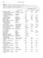
Data for solubility of inorganic substances and gases in water are given in Tables
2.3 and 2.4, respectively. Sec Refs. 1 and 3 for information on other chemical
properties of materials.
THERMOPHYSICAL PROPERTIES
Most frequently used thermophysical properties in engineering practice are
Density (
␳
)
Specific heat (c)
Specific heat at constant pressure (c
p
)
Thermal conductivity (k)
2.5
TABLE 2.2
Periodic Table of the Elements
CHAPTER TWO2.6
TABLE 2.3
Solubility of Inorganic Substances in Water
(Number of grams of the anhydrous substance soluble in 1000 g of water. The common
name of the substance is given in parentheses.)
Temperature, ЊF(ЊC)

Composition 32 (0) 122 (50) 212 (100)
Aluminum sulfate Al
2
(SO
4
)
3
313 521 891
Aluminum potassium sulfate
(potassium alum)
Al
2
K
2
(SO
4
)
4
⅐24H
2
O30 170 1540
Ammonium bicarbonate NH
4
HCO
3
119
Ammonium chloride (sal
ammoniac)
NH
4

Cl 297 504 760
Ammonium nitrate NH
4
NO
3
1183 3440 8710
Ammonium sulfate (NH
4
)
2
SO
4
706 847 1033
Barium chloride BaCl
2
⅐2H
2
O 317 436 587
Barium nitrate Ba(NO
3
)
2
50 172 345
Calcium carbonate (calcite) CaCO
3
0.018* 0.88
Calcium chloride CaCl
2
594 1576
Calcium hydroxide

(hydrated lime)
Ca(OH)
2
1.77 0.67
Calcium nitrate Ca(NO
3
)
2
⅐4H
2
O 931 3561 3626
Calcium sulfate (gypsum) CaSO
4
⅐2H
2
O 1.76 2.06 1.69
Copper sulfate (blue vitriol) CuSO
4
⅐5H
2
O 140 334 753
Ferrous chloride FeCl
2
⅐4H
2
O 644§ 820 1060
Ferrous hydroxide Fe(OH)
2
0.0067‡
Ferrous sulfate (green vitriol

or copperas)
FeSO
4
⅐7H
2
O 156 482
Ferric chloride FeCl
3
730 3160 5369
Lead chloride PbCl
2
6.73 16.7 33.3
Lead nitrate Pb(NO
3
)
2
403 1255
Lead sulfate PbSO
4
0.042†
Magnesium carbonate MgCO
3
0.13‡
Magnesium chloride MgCl
2
⅐6H
2
O 524 723
Magnesium hydroxide (milk
of magnesia)

Mg(OH)
2
0.009‡
Magnesium nitrate Mg(NO
3
)
2
⅐6H
2
O 665 903
Magnesium sulfate (Epsom
salts)
MgSO
4
⅐7H
2
O 269 500 710
Potassium carbonate (pot-
ash)
K
2
CO
3
893 1216 1562
Potassium chloride KCl 284 435 566
Potassium hydroxide (caus-
tic potash)
KOH 971 1414 1773
Potassium nitrate (saltpeter
or niter)

KNO
3
131 851 2477
Potassium sulfate K
2
SO
4
74 165 241
Sodium bicarbonate (baking
soda)
NaHCO
3
69 145
Sodium carbonate (sal soda
or soda ash)
NaCO
3
⅐10H
2
O 204 475 452
Sodium chloride (common
salt)
NaCl 357 366 392
GENERAL PROPERTIES OF MATERIALS 2.7
TABLE 2.3
Solubility of Inorganic Substances in Water (Continued )
(Number of grams of the anhydrous substance soluble in 1000 g of water. The common
name of the substance is given in parentheses.)
Temperature, ЊF(ЊC)
Composition 32 (0) 122 (50) 212 (100)

Sodium hydroxide (caustic
soda)
NaOH 420 1448 3388
Sodium nitrate (Chile salt-
peter)
NaNO
3
733 1148 1755
Sodium sulfate (Glauber
salts)
Na
2
SO
4
⅐10H
2
O49 466 422
Zinc chloride ZnCl
2
2044 4702 6147
Zinc nitrate Zn(NO
3
)
2
⅐6H
2
O 947
Zinc sulfate ZnSO
4
⅐7H

2
O 419 768 807
*59ЊF (l5ЊC).
§50
ЊF (10ЊC).
‡In cold water.
†68
ЊF (20ЊC).
Source: From Avallonc and Baumeister.
1
TABLE 2.4 Solubility of Gases in Water
(By volume, at atmospheric pressure)
t, ЊF(ЊC) 32 (0) 68 (20) 212 (100)
Air 0.032 0.020 0.012
Acetylene 1.89 1.12
Ammonia 1250 700
Carbon dioxide 1.87 0.96 0.26
Carbon monoxide 0.039 0.025
Chlorine 5.0 2.5 0.00
Hydrogen 0.023 0.020 0.018
Hydrogen sulfide 5.0 2.8 0.87
Hydrochloric acid 560 480
Nitrogen 0.026 0.017 0.0105
Oxygen 0.053 0.034 0.0185
Sulfuric acid 87 43
Source: From Avallone and Baumeister.
1
Thermal diffusivity (
␣
)

Dynamic viscosity (
␮
)
Kinematic viscosity (
␯
)
Surface tension (
␴
)
Coefficient of thermal expansion (
␤
)
The kinematic viscosity of a fluid is its dynamic viscosity divided by its density,
or
␯
ϭ
␮
/
␳
. Its units are m
2
/s. The surface tension of a fluid is the work done in
2.8
TABLE 2.5
Properties of Metallic Solids
Properties at 20
ЊC
Thermal conductivity,
k
(W/m

⅐
K)
Metal
␳
(kg/m
3
)
c
p
(J/kg
⅐
K)
k
(W/m
⅐
K)
␣
(10
Ϫ
6
m
2
/s)
Ϫ
170
ЊC
Ϫ
100
ЊC0
ЊC 100

ЊC 200
ЊC 300
ЊC 400
ЊC 600
ЊC 800
ЊC1000
ЊC
Aluminum
Pure
2,707 905 237 9.61 302 242 236
240 238 234 228 215
ϳ
95
(liq)
99% pure
211
220 206 209
Duralumin
(
ϳ
4% Cu)
2,787 883 164 6.66
126 164 182 194
Chromium
7,190 453 90 2.77 158 120 95
88 85 82 77 69 64 62
Copper and Cu alloys
Pure
8,954 384 398 11.57 483 420 401
391 389 384 378 366 352 336

Bass
(30% Zn)
8,522 385 109 3.32 73 89
106 133 143 146 147
Bronze
(25% Sn)
8,666 343 26 0.86 (Data on this and
other bronzes vary by a factor of about 2)
Constantan
(40% Ni)
8,922 410 22 0.61 17 19
22 26 35
German silver
(15% Ni, 22% Zn) 8,618 394 25 0.73
18 19 24 31 40 45 48
Gold
19,320 129 315 12.64
318 309
Ferrous metals
Pure iron
7,897 447 80 2.26 132 98
84 72 63 56 50 39 30 29.5
Cast iron
(0.4% C)
7,272 420 52 1.70
Steels
(C
Ͻ
1.5%)
0.5% carbon

(mild)
7,833 465 54 1.47
55 52 48 45 42 35 31 29
1.0% carbon 7,801 473 43 1.17
43 43 42 40 36 33 29 28
1.5% carbon 7,753 486 36 0.97
36 36 36 35 33 31 28 28
2.9
Stainless steel, type:
304
8,000 400 13.8 0.4
15 17 19 21 25
316
8,000 460 13.5 0.37
12
15 16 17 19 21 24 26
347
8,000 420 15 0.44
13
16 18 19 20 23 26 28
410
7,700 460 25 0.7
25 26 27 27 28
414
7,700 460 25 0.7
29 29
Lead
11,373 130 35 2.34 40 37
36 34 33 31 17
(liq.)

20
(liq.)
Magnesium
1,746 1023 156 8.76 17 16 157
154 152 150 148
90
(liq.)
Mercury
(polycrystalline)
32 30 7.8
(liq.)
Nickel
Pure
8,906 445 91 2.30 156 114 94
83 74 67 64 69 73 78
Nichrome
(24% Fe, 16% Cr) 8,250 448
0.34
13
Nichrome V
(20% Cr)
8,410 466 13 0.33
12 14 15 17 19
Platinum
21,450 133 71 2.50 78 73
72 72 72 73 74 77 80 84
Silver
99.99% pure 10,524 236 427 17.19
449 431 428 422 417 409 401 386 370
176

(liq.)
99.9% pure 10,524 236 411 16.55
422 405 373 367 364
Tin (polycrystalline) 7,304
ϳ
220 67 4.17 85 76 68 63
Titanium
(polycrystalline) 4,540 523 22 0.93
31 26 22 21 20 20 19 21 21
22
Tunsten
19,350 133 178 6.92 235 223 182
166 153 141 134 125 122 114
Uranium
18,700 116 28 1.29 22 24
27 29 31 33 36 41 46
Zinc
7,144 388 121 4.37 124 122 122
117 110 106 100 60
(liq.)
Source:
From Lienhard.
2
Portions of the original table have been omitted where not rele
vant to this chapter.
The data can also be found in Refs. 1, 2, and 4 through 9.
CHAPTER TWO2.10
extending the surface of a liquid one unit of area or work per unit area. Its units
are N/m. Also, note that
␣

ϭ k/
␳
c and
1
Ѩ
␳
␤
ϭϪ ϭconst
ͩͪ
p
␳
Ѩt
In general, all thermophysical properties are strong functions of temperature.
Table 2.5 shows properties of metallic solids. Table 2.6 shows properties of
nonmetallic solids. Table 2.7 shows properties of saturated liquids. (Note that the
Prandtl number Pr
ϭ
␯
/
␣
.) Table 2.8 shows properties of gases at atmospheric
pressure. Table 2.9 shows data of surface tension of various liquids. Approximate
relations for thermal expansions are given in Table 2.14.
MECHANICAL PROPERTIES
Mechanical properties commonly used by engineers are
Ultimate tensile strength
Tensile yield strength
Elongation
Modulus of elasticity
Compressive strength

Shear strength
Endurance limit
Ultimate tensile strength is defined as the maximum load per unit of original
cross-sectional area sustained by a material during a tension test. It is also called
ultimate strength.
Tensile yield strength is defined as the stress corresponding to some permanent
deformation from the modulus slope, e.g., 0.2 percent offset in the case of heat-
treated alloy steels.
Elongation is defined as the amount of permanent extension in a ruptured tensile
test specimen; it is usually expressed as a percentage of the original gage length.
Elongation is usually taken as a measure of ductility.
Modulus of elasticity is the property of a material which indicates its rigidity.
This property is the ratio of stress to strain within the elastic range.
On a stress-strain diagram, the modulus of elasticity is usually represented by
the straight portion of the curve when the stress is directly proportional to the strain.
The steeper the curve, the higher the modulus of elasticity and the stiffer the ma-
terial.
Compressive strength is defined as the maximum compressive stress that a ma-
terial is capable of developing based on the original cross-sectional area. The gen-
eral design practice is to assume the compressive strength of a steel is equal to its
tensile strength, although it is actually somewhat greater.
Shear strength is defined as the stress required to produce fracture in the plane
of cross section, the conditions of loading being such that the directions of force
and of resistance are parallel and opposite although their paths are offset a specified
minimum amount. The ultimate shear strength is generally assumed to be three-
fourths the material’s ultimate tensile strength.
GENERAL PROPERTIES OF MATERIALS 2.11
TABLE 2.6
Properties of Nonmetallic Solids
Material

Tem-
perature
range,
ЊC
Density
␳
,
kg/m
3
Specific
heat c,
J/kg
⅐ ЊC
Thermal
conduc-
tivity k,
W/m
⅐ ЊC
Thermal
diffusivity
␣
,m
2
/s
Asbestos
Cement board 20 0.6
Fiber (properties vary 20 1930 0.8
with packing) 20 980 0.14
Asphalt 20–25 0.75
Beef 25 1.35

ϫ 10
07
Brick
B&W, K-28 insulating 300 0.3
B&W, K-28 insulating 1000 0.4
Cement 10 720 0.34
Common 0–1000 0.7
Chrome 100 1.9
Firebrick 300 2000 960 0.1 5.4
ϫ 10
Ϫ
8
Firebrick 1000 0.2
Carbon
Diamond (type II b) 20
ϳ3250 510 1350. 8.1 ϫ 10
Ϫ
4
Graphite 20 ϳ2100 ϳ2090 Highly variable structure
Cardboard 0–20 790 0.14
Clay
Fireclay 500–750 1.
Sandy clay 20 1780 0.9
Coal
Anthracite 900
ϳ1500 ϳ0.2
Brown coal 900
ϳ0.1
Bituminous in situ
ϳ1300 0.5–0.7 3 to 4 ϫ 10

Ϫ
7
Concrete
Limestone gravel 20 1850 0.6
Portland cement 90 2300 1.7
Sand:cement (3:1) 230 0.1
Slag cement 20 0.14
Corkboard (medium
␳
)30170 0.04
Egg white 20 1.37
ϫ 10
Ϫ
7
Glass
Lead 36 1.2
Plate 20 1.3
Pyrex 60–100 2210 753 1.3 7.8
ϫ 10
Ϫ
7
Soda 20 0.7
Window 46 1.3
Glass wool 20 64–160 0.04
Ice 0 917 2100 2.215 1.15
ϫ 10
Ϫ
6
Ivory 80 0.5
Kapok 30 0.035

CHAPTER TWO2.12
TABLE 2.6
Properties of Nonmetallic Solids (Continued )
Material
Tem-
perature
range,
ЊC
Density
␳
,
kg/m
3
Specific
heat c,
J/kg
⅐ ЊC
Thermal
conduc-
tivity k,
W/m
⅐ ЊC
Thermal
diffusivity
␣
,m
2
/s
Magnesia (85%) 38 0.067
93 0.071

150 0.074
204 0.08
Lunar surface dust
(high vacuum)
250 1500
ע 300 ϳ600 ϳ0.0006 ϳ7 ϫ 10
Ϫ
10
Rock wool Ϫ5 ϳ130 0.03
93 0.05
Rubber (hard) 0 1200 2010 0.15 6.2
ϫ 10
Ϫ
8
Silica aerogel 0 140 0.024
120 136 0.022
Silo-cel (diatomaceous
earth)
0 320 0.061
Soil (mineral)
Dry 15 1500 1840 1. 4
ϫ 10
Ϫ
7
Wet151930 2.
Stone
Granite (NTS) 20
ϳ2640 ϳ820 1.6 ϳ7.4 ϫ 10
Ϫ
7

Limestone (Indiana) 100 2300 ϳ900 1.1 ϳ5.3 ϫ 10
Ϫ
7
Sandstone (Berea) 25 ϳ3
Slate 100 1.5
Wood (perpendicular to
grain)
Ash 15 740 0.15–0.3
Balsa 15 100 0.05
Cedar 15 480 0.11
Fir 15 600 2720 0.12 7.4
ϫ 10
Ϫ
8
Mahogany 20 700 0.16
Oak 20 600 2390 0.1–0.4 (0.7–2.8)
ϫ 10
Ϫ
7
Pitch pine 20 450 0.14
Sawdust (dry) 17 128 0.14
Spruce 20 410 0.11
Wool (sheep) 20 145 0.05
Source: From Lienhard.
2
Portions of the original table have been omitted where not relevant to this
chapter. The data can also be found in Refs. 1, 2, and 4 through 9.
Endurance limit is defined as the maximum stress to which the material can be
subjected for an indefinite service life. Although the standards vary for various
types of members and different industries, it is common practice to assume that

carrying a certain load for several million cycles of stress reversals indicates that
the load can be carried for an indefinite time.
Hardness measures the resistance of the material to indentation. Hardness tests
measure the plastic deformation (the size or depth) of an indentation. Brinell hard-
GENERAL PROPERTIES OF MATERIALS 2.13
TABLE 2.7
Thermophysical Properties of Saturated Liquids
Temp.,
K ЊC
␳
,
kg/m
3
c
p
,
J/kg
⅐ K
k,
W/m ⅐ K
␣
,m
2
/s
␯
,m
2
/s Pr
␤
,

K
Ϫ
1
Ammonia (there is considerable disagreement among sources)
220 Ϫ53 706 4426 0.66 2.11 ϫ 10
Ϫ
7
240 Ϫ33 682 4484 0.61 2.00 4.17 ϫ 10
Ϫ
7
2.09
260
Ϫ13 656 4547 0.57 1.91 3.27 1.71
280 7 629 4625 0.52 1.79 2.68 1.50 0.00025
300 27 600 4736 0.470 1.65 2.32 1.41
320 47 568 4962 0.424 1.50 2.06 1.37
340 67 533 5214 0.379 1.36 1.79 1.32
360 87 490 5635 0.335 1.21 1.55 1.28
380 107 436 0.289 1.34
400 127 345 0.245 1.19
CO
2
250 Ϫ23 1046 1990 0.135 6.49 ϫ 10
Ϫ
8
260 Ϫ13 998 2110 0.123 5.84 1.15 ϫ 10
Ϫ
7
1.97
270

Ϫ3 944 2390 0.113 5.09 1.08 2.12
280 7 883 2760 0.102 4.19 1.04 2.48
290 17 805 3630 0.090 3.08 0.99 3.20 0.014
300 27 676 7690 0.076 1.46 0.88 6.04
303 30 604
D
2
O (heavy water)
589 316 740 2034 0.0509 0.978 ϫ 10
Ϫ
7
1.23 ϫ 10
Ϫ
7
1.257
Freon 11 (trichlorofluoromethane)
220 Ϫ53 829 0.110
240
Ϫ33 1607 841 0.105 7.8 ϫ 10
Ϫ
8
4.78 ϫ 10
Ϫ
7
6.1
260
Ϫ13 1564 855 0.099 7.4 4.10 5.5
280 7 1518 871 0.093 7.0 3.81 5.4 0.00154
300 27 1472 888 0.088 6.7 2.82 4.2 0.00163
320 47 1421 906 0.082 6.4

340 67 1369 927 0.076 6.0
Freon 12 (dichlorodifluoromethane)
160 Ϫ113 0.133
180
Ϫ93 1664 834 0.124 8.935 ϫ 10
Ϫ
8
200 Ϫ73 1610 856 0.1148 8.33
220
Ϫ53 1555 873 0.1057 7.79 3.2 ϫ 10
Ϫ
7
4.11 0.00263
240
Ϫ33 1498 892 0.0965 7.22 2.60 3.60
260
Ϫ13 1438 914 0.0874 6.65 2.26 3.40
280 7 1374 942 0.0782 6.04 2.06 3.41
300 27 1305 980 0.0690 5.39 1.95 3.62
320 47 1229 1031 0.0599 4.72 1.9 4.03
340 67 1097 0.0507
Glycerin (or glycerol)
273 0 1276 2200 0.282 1.00 ϫ 10
Ϫ
7
0.0083 83,000
293 20 1261 2350 0.285 0.962 0.001120 11,630 0.00048
303 30 1255 2400 0.285 0.946 0.000488 5,161 0.00049
313 40 1249 2460 0.285 0.928 0.000227 2,451 0.00049
323 50 1243 2520 0.285 0.910 0.000114 1,254 0.00050

CHAPTER TWO2.14
TABLE 2.7
Thermophysical Properties of Saturated Liquids (Continued )
Temp.,
K ЊC
␳
,
kg / m
3
c
p
,
J/kg
⅐ K
k,
W/m ⅐ K
␣
,m
2
/s
␯
,m
2
/s Pr
␤
,
K
Ϫ
1
Glycerin (or glycerol) (Continued )

644 371 10,540 159 16.1 1.084 ϫ 10
Ϫ
5
2.276 ϫ 10
Ϫ
7
0.024
755 482 10,442 155 15.6 1.223 1.85 0.017
811 538 10,348 145 15.3 1.02 1.68 0.017
Mercury
234 Ϫ39 141.5 6.97 3.62 ϫ 10
Ϫ
6
250 Ϫ23 140.5 7.32 3.83
300 27 13,611 139.1 8.34 4.41 1.2
ϫ 10
Ϫ
7
0.027
350 77 3,489 137.7 5.29 4.91 1.0 0.020
400 127 13,367 136.7 5.69 5.83
ϫ 10
Ϫ
6
0.95 ϫ 10
Ϫ
7
0.016
500 277 13,128 135.6 6.36 6.00 0.80 0.013
600 327 135.4 6.93 6.55 0.68 0.010

700 427 136.1 7.34
800 527 7.40
Methyl alcohol (methanol)
260 Ϫ13 823 2336 0.2164 1.126 ϫ 10
Ϫ
7
Ϫ1.3 ϫ 10
Ϫ
6
ϳ11.5
280 7 804 2423 0.2078 1.021
ϳ0.9 ϳ8.8 0.00114
300 27 785 2534 0.2022 1.016
ϳ0.7 ϳ6.9
320 47 767 2672 0.1965 0.959
ϳ0.6 ϳ6.3
340 67 748 2856 0.1908 0.893
ϳ0.44 ϳ4.9
360 87 729 3036 0.1851 0.836
ϳ0.36 ϳ4.3
380 107 710 3265 0.1794 0.774
ϳ0.30 ϳ4.1
Oxygen
54 1276 1648 0.191 9.08 ϫ 10
Ϫ
8
6.5 ϫ 10
Ϫ
7
7.15

60
Ϫ213 1649 0.185
80
Ϫ193 1653 0.1623
90
Ϫ183 1114 1655 0.1501 8.14 ϫ 10
Ϫ
8
1.75 ϫ 10
Ϫ
7
2.15
120
Ϫ153 0.1096
150
Ϫ123 0.061
Oils (some approximate viscosities)
273 0 MS-20 0.0076 100,000
339 66 California crude (heavy) 0.00008
289 16 California crude (light) 0.00005
339 66 California crude (light) 0.000010
289 16 Light machine oil 0.0007
339 66 Light machine oil 0.00004
289 16 Light machine oil (
␳
ϭ 907) 0.00016
339 66 Light machine oil (
␳
ϭ 907) 0.000013
289 16 SAE 30 0.00044

Ϫ5,000
339 66 SAE 30 0.00003
289 16 SAE 30 (Eastern) 0.00011
339 66 SAE 30 (Eastern) 0.00001
289 16 Spindle oil (
␳
ϭ 885) 0.00005
339 66 Spindle oil (
␳
ϭ 885) 0.000007
GENERAL PROPERTIES OF MATERIALS 2.15
TABLE 2.7
Thermophysical Properties of Saturated Liquids (Continued )
Temp.,
K ЊC
␳
,
kg/m
3
c
p
,
J/kg
⅐ K
k,
W/m ⅐ K
␣
,m
2
/s

␯
,m
2
/s Pr
␤
,
K
Ϫ
1
Water
273 0 999.8 4205 0.5750 1.368 ϫ 10
Ϫ
7
1.753 ϫ 10
Ϫ
6
12.81
280 7 999.9 4196 0.5818 1.386 1.422 10.26
300 27 996.6 4177 0.6084 1.462 0.826 5.65 0.000275
320 47 989.3 4177 0.6367 1.541
ϫ 10
Ϫ
7
0.566 ϫ 10
Ϫ
6
3.67 0.000435
340 67 979.5 4187 0.6587 1.606 0.420 2.61
360 87 967.4 4206 0.6743 1.657 0.330 1.99
373 100 957.2 4219 0.6811 1.683 0.290 1.72

400 127 937.5 4241 0.6864 1.726 0.229 1.33
420 147 919.9 4306 0.6836 1.726
ϫ 10
Ϫ
7
2.000 ϫ 10
Ϫ
7
1.16
440 167 900.5 4391 0.6774 1.713 1.786 1.04
460 187 879.5 4456 0.6672 1.703 1.626 0.955
480 207 856.6 4534 0.6530 1.681 1.504 0.894
500 227 831.5 4647 0.6348 1.463 1.412 0.859
520 247 803.9 4831 0.6123 1.577
ϫ 10
Ϫ
7
1.345 ϫ 10
Ϫ
7
0.853
540 267 773.0 5099 0.5857 1.486 1.298 0.873
560 287 738.2 5487 0.555 1.370 1.269 0.926
580 307 697.6 6010 0.520 1.240 1.240 1.000
600 327 648.8 6691 0.481 1.108 1.215 1.097
620 347 586.3 1.213
ϫ 10
Ϫ
7
640 367 482.1 1.218

647.3 374.2 306.8 1.356
Source: From Lienhard. Portions of the original table have been omitted where not relevant to this
chapter. The data can also be found in Refs. 1. 2, and 4 through 9.
ness tests use spheres as indenters; the Vickers test uses pyramids. Rockwell tests
use cones or spheres. Microhardness tests for specimens are also available, using
the Knoop method with miniature pyramid indenters. Another hardness scale is
Mohs’ scale, which lists materials in order of their hardness, beginning with talc
and ending with diamond. Table 2.15 shows typical Brinell hardness number (BHN)
for metals.
Table 2.10 shows typical mechanical properties of some metals and alloys. See
Ref. 11 for more data.
Note on Hardness Testing Method
Hardness tests on materials consist of pressing a hardened ball point into a specimen
and measuring the size of the resulting indentation (see Figure 2.1). The method
shown is the Brinell method, which utilizes a ball. The ball size is 10 mm for most
cases or 1 mm for light work.
Let:
D
ϭ diameter of indentation (mm)
D
ϭ diameter of baIl (mm)
b
F ϭ force on ball (kg )
f
(continues on page 2.22)