Data Mining and Knowledge Discovery Handbook, 2 Edition part 130 doc

1270
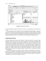
Fig. 66.1. The Explorer Interface.
to compare different methods and identify those that are most appropriate for the problem at
hand.
The workbench includes methods for all the standard Data Mining problems: regression,
classification, clustering, association rule mining, and attribute selection. Getting to know the
data is is a very important part of Data Mining, and many data visualization facilities and data
preprocessing tools are provided. All algorithms and methods take their input in the form of a
single relational table, which can be read from a file or generated by a database query.
Exploring the Data
The main graphical user interface, the “Explorer,” is shown in Figure 66.1. It has six differ-
ent panels, accessed by the tabs at the top, that correspond to the various Data Mining tasks
supported. In the “Preprocess” panel shown in Figure 66.1, data can be loaded from a file
or extracted from a database using an SQL query. The file can be in CSV format, or in the
system’s native ARFF file format. Database access is provided through Java Database Con-
nectivity, which allows SQL queries to be posed to any database for which a suitable driver
exists. Once a dataset has been read, various data preprocessing tools, called “filters,” can be
applied—for example, numeric data can be discretized. In Figure 66.1 the user has loaded a
data file and is focusing on a particular attribute, normalized-losses, examining its statistics
and a histogram.
Through the Explorer’s second panel, called “Classify,” classification and regression al-
gorithms can be applied to the preprocessed data. This panel also enables users to evaluate
the resulting models, both numerically through statistical estimation and graphically through
visualization of the data and examination of the model (if the model structure is amenable to
visualization). Users can also load and save models.
Eibe Frank et al.
66 Weka-A Machine Learning Workbench for Data Mining 1271
Fig. 66.2. The Knowledge Flow Interface.
The third panel, “Cluster,” enables users to apply clustering algorithms to the dataset.
Again the outcome can be visualized, and, if the clusters represent density estimates, evalu-
ated based on the statistical likelihood of the data. Clustering is one of two methodologies

for analyzing data without an explicit target attribute that must be predicted. The other one
comprises association rules, which enable users to perform a market-basket type analysis of
the data. The fourth panel, “Associate,” provides access to algorithms for learning association
rules.
Attribute selection, another important Data Mining task, is supported by the next panel.
This provides access to various methods for measuring the utility of attributes, and for finding
attribute subsets that are predictive of the data. Users who like to analyze the data visually are
supported by the final panel, “Visualize.” This presents a color-coded scatter plot matrix, and
users can then select and enlarge individual plots. It is also possible to zoom in on portions of
the data, to retrieve the exact record underlying a particular data point, and so on.
The Explorer interface does not allow for incremental learning, because the Preprocess
panel loads the dataset into main memory in its entirety. That means that it can only be used for
small to medium sized problems. However, some incremental algorithms are implemented that
can be used to process very large datasets. One way to apply these is through the command-line
interface, which gives access to all features of the system. An alternative, more convenient,
approach is to use the second major graphical user interface, called “Knowledge Flow.” Il-
lustrated in Figure 66.2, this enables users to specify a data stream by graphically connecting
components representing data sources, preprocessing tools, learning algorithms, evaluation
methods, and visualization tools. Using it, data can be processed in batches as in the Explorer,
or loaded and processed incrementally by those filters and learning algorithms that are capable
of incremental learning.
An important practical question when applying classification and regression techniques is
to determine which methods work best for a given problem. There is usually no way to answer
1272
Fig. 66.3. The Experimenter Interface.
this question a priori, and one of the main motivations for the development of the workbench
was to provide an environment that enables users to try a variety of learning techniques on a
particular problem. This can be done interactively in the Explorer. However, to automate the
process Weka includes a third interface, the “Experimenter,” shown in Figure 66.3. This makes
it easy to run the classification and regression algorithms with different parameter settings on a

corpus of datasets, collect performance statistics, and perform significance tests on the results.
Advanced users can also use the Experimenter to distribute the computing load across multiple
machines using Java Remote Method Invocation.
Methods and Algorithms
Weka contains a comprehensive set of useful algorithms for a panoply of Data Mining tasks.
These include tools for data engineering (called “filters”), algorithms for attribute selection,
clustering, association rule learning, classification and regression. In the following subsections
we list the most important algorithms in each category. Most well-known algorithms are in-
cluded, along with a few less common ones that naturally reflect the interests of our research
group.
An important aspect of the architecture is its modularity. This allows algorithms to be
combined in many different ways. For example, one can combine bagging! boosting, decision
tree learning and arbitrary filters directly from the graphical user interface, without having to
write a single line of code. Most algorithms have one or more options that can be specified.
Explanations of these options and their legal values are available as built-in help in the graphi-
cal user interfaces. They can also be listed from the command line. Additional information and
pointers to research publications describing particular algorithms may be found in the internal
Javadoc documentation.
Eibe Frank et al.
66 Weka-A Machine Learning Workbench for Data Mining 1273
Classification
Implementations of almost all main-stream classification algorithms are included. Bayesian
methods include naive Bayes, complement naive Bayes, multinomial naive Bayes, Bayesian
networks, and AODE. There are many decision tree learners: decision stumps, ID3, a C4.5
clone called “J48,” trees generated by reduced error pruning, alternating decision trees, and
random trees and forests thereof. Rule learners include OneR, an implementation of Ripper
called “JRip,” PART, decision tables, single conjunctive rules, and Prism. There are several
separating hyperplane approaches like support vector machines with a variety of kernels, lo-
gistic regression, voted perceptrons, Winnow and a multi-layer perceptron. There are many
lazy learning methods like IB1, IBk, lazy Bayesian rules, KStar, and locally-weighted learn-

ing.
As well as the basic classification learning methods, so-called
“meta-learning” schemes enable users to combine instances of one or more of the basic al-
gorithms in various ways: bagging! boosting (including the variants AdaboostM1 and Logit-
Boost), and stacking. A method called “FilteredClassifier” allows a filter to be paired up with a
classifier. Classification can be made cost-sensitive, or multi-class, or ordinal-class. Parameter
values can be selected using cross-validation.
Regression
There are implementations of many regression schemes. They include simple and multiple
linear regression, pace regression, a multi-layer perceptron, support vector regression, locally-
weighted learning, decision stumps, regression and model trees (M5) and rules (M5rules). The
standard instance-based learning schemes IB1 and IBk can be applied to regression problems
(as well as classification problems). Moreover, there are additional meta-learning schemes that
apply to regression problems, such as additive regression and regression by discretization.
Clustering
At present, only a few standard clustering algorithms are included: KMeans, EM for naive
Bayes models, farthest-first clustering, and Cobweb. This list is likely to grow in the near
future.
Association rule learning
The standard algorithm for association rule induction is Apriori, which is implemented in
the workbench. Two other algorithms implemented in Weka are Tertius, which can extract
first-order rules, and Predictive Apriori, which combines the standard confidence and support
statistics into a single measure.
Attribute selection
Both wrapper and filter approaches to attribute selection are supported. A wide range of fil-
tering criteria are implemented, including correlation-based feature selection, the chi-square
statistic, gain ratio, information gain, symmetric uncertainty, and a support vector machine-
based criterion. There are also a variety of search methods: forward and backward selection,
best-first search, genetic search, and random search. Additionally, principal components anal-
ysis can be used to reduce the dimensionality of a problem.

1274
Filters
Processes that transform instances and sets of instances are called “filters,” and they are clas-
sified according to whether they make sense only in a prediction context (called “supervised”)
or in any context (called “unsupervised”). We further split them into “attribute filters,” which
work on one or more attributes of an instance, and “instance filters,” which manipulate sets of
instances.
Unsupervised attribute filters include adding a new attribute, adding a cluster indicator,
adding noise, copying an attribute, discretizing a numeric attribute, normalizing or standard-
izing a numeric attribute, making indicators, merging attribute values, transforming nominal
to binary values, obfuscating values, swapping values, removing attributes, replacing miss-
ing values, turning string attributes into nominal ones or word vectors, computing random
projections, and processing time series data. Unsupervised instance filters transform sparse
instances into non-sparse instances and vice versa, randomize and resample sets of instances,
and remove instances according to certain criteria.
Supervised attribute filters include support for attribute selection, discretization, nominal
to binary transformation, and re-ordering the class values. Finally, supervised instance filters
resample and subsample sets of instances to generate different class distributions—stratified,
uniform, and arbitrary user-specified spreads.
System Architecture
In order to make its operation as flexible as possible, the workbench was designed with a mod-
ular, object-oriented architecture that allows new classifiers, filters, clustering algorithms and
so on to be added easily. A set of abstract Java classes, one for each major type of component,
were designed and placed in a corresponding top-level package.
All classifiers reside in subpackages of the top level “classifiers” package and extend a
common base class called “Classifier.” The Classifier class prescribes a public interface for
classifiers and a set of conventions by which they should abide. Subpackages group compo-
nents according to functionality or purpose. For example, filters are separated into those that
are supervised or unsupervised, and then further by whether they operate on an attribute or
instance basis. Classifiers are organized according to the general type of learning algorithm,

so there are subpackages for Bayesian methods, tree inducers, rule learners, etc.
All components rely to a greater or lesser extent on supporting classes that reside in a
top level package called “core.” This package provides classes and data structures that read
data sets, represent instances and attributes, and provide various common utility methods. The
core package also contains additional interfaces that components may implement in order to
indicate that they support various extra functionality. For example, a classifier can implement
the “WeightedInstancesHandler” interface to indicate that it can take advantage of instance
weights.
A major part of the appeal of the system for end users lies in its graphical user inter-
faces. In order to maintain flexibility it was necessary to engineer the interfaces to make it as
painless as possible for developers to add new components into the workbench. To this end,
the user interfaces capitalize upon Java’s introspection mechanisms to provide the ability to
configure each component’s options dynamically at runtime. This frees the developer from
having to consider user interface issues when developing a new component. For example, to
enable a new classifier to be used with the Explorer (or either of the other two graphical user
Eibe Frank et al.
66 Weka-A Machine Learning Workbench for Data Mining 1275
interfaces), all a developer need do is follow the Java Bean convention of supplying “get” and
“set” methods for each of the classifier’s public options.
Applications
Weka was originally developed for the purpose of processing agricultural data, motivated by
the importance of this application area in New Zealand. However, the machine learning meth-
ods and data engineering capability it embodies have grown so quickly, and so radically, that
the workbench is now commonly used in all forms of Data Mining applications—from bioin-
formatics to competition datasets issued by major conferences such as Knowledge Discovery
in Databases.
New Zealand has several research centres dedicated to agriculture and horticulture, which
provided the original impetus for our work, and many of our early applications. For exam-
ple, we worked on predicting the internal bruising sustained by different varieties of apple
as they make their way through a packing-house on a conveyor belt (Holmes et al., 1998);

predicting, in real time, the quality of a mushroom from a photograph in order to provide
automatic grading (Kusabs et al., 1998); and classifying kiwifruit vines into twelve classes,
based on visible-NIR spectra, in order to determine which of twelve pre-harvest fruit man-
agement treatments has been applied to the vines (Holmes and Hall, 2002). The applicability
of the workbench in agricultural domains was the subject of user studies (McQueen et al.,
1998) that demonstrated a high level of satisfaction with the tool and gave some advice on
improvements.
There are countless other applications, actual and potential. As just one example, Weka
has been used extensively in the field of bioinformatics. Published studies include automated
protein annotation (Bazzan et al., 2002), probe selection for gene expression arrays (Tobler
et al., 2002), plant genotype discrimination (Taylor et al., 2002), and classifying gene expres-
sion profiles and extracting rules from them (Li et al., 2003). Text mining is another major
field of application, and the workbench has been used to automatically extract key phrases
from text (Frank et al., 1999), and for document categorization (Sauban and Pfahringer, 2003)
and word sense disambiguation (Pedersen, 2002).
The workbench makes it very easy to perform interactive experiments, so it is not sur-
prising that most work has been done with small to medium sized datasets. However, larger
datasets have been successfully processed. Very large datasets are typically split into several
training sets, and a voting-
committee structure is used for prediction. The recent development of the knowledge flow
interface should see larger scale application development, including online learning from
streamed data.
Many future applications will be developed in an online setting. Recent work on data
streams (Holmes et al., 2003) has enabled machine learning algorithms to be used in situations
where a potentially infinite source of data is available. These are common in manufacturing
industries with 24/7 processing. The challenge is to develop models that constantly monitor
data in order to detect changes from the steady state. Such changes may indicate failure in
the process, providing operators with warning signals that equipment needs re-calibrating or
replacing.
1276

Summing up the Workbench
Weka has three principal advantages over most other Data Mining software. First, it is open
source, which not only means that it can be obtained free, but—more importantly—it is main-
tainable, and modifiable, without depending on the commitment, health, or longevity of any
particular institution or company. Second, it provides a wealth of state-of-the-art machine
learning algorithms that can be deployed on any given problem. Third, it is fully implemented
in Java and runs on almost any platform—even a Personal Digital Assistant.
The main disadvantage is that most of the functionality is only applicable if all data is held
in main memory. A few algorithms are included that are able to process data incrementally or
in batches (Frank et al., 2002). However, for most of the methods the amount of available
memory imposes a limit on the data size, which restricts application to small or medium-
sized datasets. If larger datasets are to be processed, some form of subsampling is generally
required. A second disadvantage is the flip side of portability: a Java implementation may be
somewhat slower than an equivalent in C/C++.
Acknowledgments
Many thanks to past and present members of the Waikato machine learning group and the
many external contributors for all the work they have put into Weka.
References
Bazzan, A. L., Engel, P. M., Schroeder, L. F., and da Silva, S. C. (2002). Automated an-
notation of keywords for proteins related to mycoplasmataceae using machine learning
techniques. Bioinformatics, 18:35S–43S.
Frank, E., Holmes, G., Kirkby, R., and Hall, M. (2002). Racing committees for large datasets.
In Proceedings of the International Conference on Discovery Science, pages 153–164.
Springer-Verlag.
Frank, E., Paynter, G. W., Witten, I. H., Gutwin, C., and Nevill-Manning, C. G. (1999).
Domain-specific keyphrase extraction. In Proceedings of the 16th International Joint
Conference on Artificial Intelligence, pages 668–673. Morgan Kaufmann.
Holmes, G., Cunningham, S. J., Rue, B. D., and Bollen, F. (1998). Predicting apple bruising
using machine learning. Acta Hort, 476:289–296.
Holmes, G. and Hall, M. (2002). A development environment for predictive modelling in

foods. International Journal of Food Microbiology, 73:351–362.
Holmes, G., Kirkby, R., and Pfahringer, B. (2003). Mining data streams using option trees.
Technical Report 08/03, Department of Computer Science, University of Waikato.
Kusabs, N., Bollen, F., Trigg, L., Holmes, G., and Inglis, S. (1998). Objective measurement
of mushroom quality. In Proc New Zealand Institute of Agricultural Science and the
New Zealand Society for Horticultural Science Annual Convention, page 51.
Li, J., Liu, H., Downing, J. R., Yeoh, A. E J., and Wong, L. (2003). Simple rules underlying
gene expression profiles of more than six subtypes of acute lymphoblastic leukemia (all)
patients. Bioinformatics, 19:71–78.
McQueen, R., Holmes, G., and Hunt, L. (1998). User satisfaction with machine learning as
a data analysis method in agricultural research. New Zealand Journal of Agricultural
Research, 41(4):577–584.
Eibe Frank et al.
66 Weka-A Machine Learning Workbench for Data Mining 1277
Pedersen, T. (2002). Evaluating the effectiveness of ensembles of decision trees in disam-
biguating Senseval lexical samples. In Proceedings of the ACL-02 Workshop on Word
Sense Disambiguation: Recent Successes and Future Directions.
Sauban, M. and Pfahringer, B. (2003). Text categorisation using document profiling. In
Proceedings of the 7th European Conference on Principles and Practice of Knowledge
Discovery in Databases, pages 411–422. Springer.
Taylor, J., King, R. D., Altmann, T., and Fiehn, O. (2002). Application of metabolomics
to plant genotype discrimination using statistics and machine learning. Bioinformatics,
18:241S–248S.
Tobler, J. B., Molla, M., Nuwaysir, E., Green, R., and Shavlik, J. (2002). Evaluating machine
learning approaches for aiding probe selection for gene-expression arrays. Bioinformat-
ics, 18:164S–171S.

Index
A*, 897
Accuracy, 617

AdaBoost, 754, 882, 883, 962, 974, 1273
Adaptive piecewise constant approximation,
1069
Aggregation operators, 1000–1004
AIC (Akaike information criterion), 96, 214,
536, 564, 644, 1211
Akaike information criterion (AIC), 96, 214,
536, 564, 644, 1211
Anomaly detection, 1050, 1063
Anonymity preserving pattern discovery,
689
Apriori, 324, 1013, 1172
Arbiter tree, 969, 970, 973, 974
Area under the curve (AUC), 156, 877, 878
ARIMA (Auto regressive integrated moving
average), 122, 527, 1154, 1156
Association Rules, 604
Association rules, 24, 26, 110, 300, 301,
307, 313–315, 321, 339, 436, 528,
533, 535, 536, 541, 543, 548, 549,
603, 605–607, 614, 620, 622–624,
653, 655, 656, 659, 662, 826, 846,
901, 1012, 1014, 1023, 1032, 1126,
1127, 1172, 1175, 1177, 1271
relational, 888, 890, 899, 901
Association rules,relational, 899
Attribute, 134, 142
domain, 134
input, 133
nominal, 134, 150

numeric, 134, 150
target, 133
Attribute-based learning methods, 1154
AUC (Area Under the Curve), 156, 877, 878
Auto regressive integrated moving average
(ARIMA), 122, 527, 1154, 1156
AUTOCLASS, 283
Average-link clustering, 279
Bagging, 209, 226, 645, 744, 801, 881, 960,
965, 966, 973, 1004, 1211, 1272, 1273
Bayes factor, 183
Bayes’ theorem, 182
Bayesian combination, 967
Bayesian information criterion (BIC), 96,
182, 195, 295, 644, 1211
Bayesian model selection, 181
Bayesian Networks
dynamic, 196
Bayesian networks, 88, 95, 175, 176, 178,
182, 191, 203, 1128, 1273
dynamic, 195, 197
Bayesware Discoverer, 189
Bias, 734
BIC (Bayesian information criterion), 96,
182, 195, 295, 644, 1211
Bioinformatics, 1154
Blanket residuals, 189
Bonferonni coefficient, 1211
Boosting, 80, 229, 244, 645, 661, 725, 744,
754, 755, 801, 818, 881, 882, 962,

1004, 1030, 1211, 1272
Bootstraping, 616
BPM (Business performance management),
1043
O. Maimon, L. Rokach (eds.), Data Mining and Knowledge Discovery Handbook, 2nd ed.,
DOI 10.1007/978-0-387-09823-4, © Springer Science+Business Media, LLC 2010
1280 Index
Business performance management (BPM),
1043
C-medoids, 480
C4.5, 34, 88, 92, 94, 112, 135, 151, 163,
795, 798, 881, 899, 907, 961, 972,
1012, 1118, 1198, 1273
CART, 510
CART (Classification and regression trees),
34, 151, 163, 164, 220, 222, 224–226,
899, 907, 987, 990, 1118, 1198
Case-based reasoning (CBR), 1121
Category connection map, 822
Category utility metric, 276
Causal networks, 949
Centering, 71
CHAID, 164
Chebychev metric, 270
Classifer
crisp, 136
probabilistic, 136
Classification, 22, 92, 191, 203, 227, 233,
378, 384, 394, 419, 429, 430, 507,
514, 532, 563, 617, 646, 735, 806,

1004, 1124
accuracy, 136
hypertext, 917
problem definition, 135
text, 245, 818, 914, 917, 920, 921
time series, 1050
Classifier, 53, 133, 135, 660, 661, 748, 816,
876, 878, 1122
probabilistic, 817
Closed Frequent Sets, 332
Clustering, 25, 381, 382, 419, 433, 510, 514,
515, 562, 932
complete-link, 279
crisp, 630, 934
fuzzy, 285, 934, 938
graph-based, 934, 937
hierarchical, 934, 935
link-based, 939
neural network, 934, 938
partitional, 934
probabilistic, 934, 939
spectral, 77, 78
time series, 1050, 1059
Clustering,fuzzy, 635
COBWEB, 284, 291, 1273
Combiner tree, 971
Comprehensibility, 136, 140, 984
Computational complexity, 140
Concept, 134
Concept class, 135

Concept learning, 134
Conditional independence, 177
Condorcet’s criterion, 276
Confidence, 621
Configuration, 182
Connected component, 1092
Consistency, 137
Constraint-based Data Mining, 340
Conviction, 623
Cophenetic correlation coefficient, 628
Cosine distance, 935, 1197
Cover, 322
Coverage, 621
CRISP-DM (CRoss Industry Standard
Process for Data Mining), 1032, 1033,
1047, 1112
CRM (Customer relationship management),
1043, 1181, 1189
Cross-validation, 139, 190, 526, 564, 616,
645, 724, 966, 1122, 1211, 1273
Crossover
commonality-based crossover, 396
Customer relationship management (CRM),
1043, 1181, 1189
Data cleaning, 19, 615
Data collection, 1084
Data envelop analysis (DEA), 968
Data management, 559
Data mining, 1082
Data Mining Tools, 1155

Data reduction, 126, 349, 554, 566, 615
Data transformation, 561, 615, 1172
Data warehouse, 20, 141, 1010, 1118, 1179
Database, 1084
DBSCAN, 283
DEA (Data envelop analysis), 968
Decision support systems, 566, 718, 1043,
1046, 1122, 1166
Decision table majority, 89, 94
Decision tree, 133, 149, 151, 284, 391, 509,
961, 962, 964, 967, 972, 974, 1011,
1117
internal node, 149
Index 1281
leaf, 149
oblivious, 167
test node, 149
Decomposition, 981
concept aggregation, 985
feature set, 987
function, 985
intermediate concept, 985, 992
Decomposition,original concept, 992
Dempster–Shafer, 967
Denoising, 560
Density-based methods, 278
Design of experiments, 1187
Determinant criterion, 275
Dimensionality reduction, 53, 54, 143, 167,
559, 561, 939, 1004, 1057, 1060, 1063

Directed acyclic graph, 176
Directed hyper-Markov law, 182
Directed tree, 149
Dirichlet distribution, 185
Discrete fourier transform (DFT), 1066
Discrete wavelet transform (DWT), 555,
1067
Distance measure, 123, 155, 270, 311, 615,
1050, 1122, 1174, 1197
dynamic time warping, 1051
Euclidean, 1050
Distortion discriminant analysis, 66
Distributed Data Mining, 564, 993, 1024
Distribution summation, 967
Dynamic time warping, 1051
Eclat, 327
Edge cut metrics, 277
Ensemble methods, 226, 744, 881, 959, 990,
1004
Entropy, 153, 968
Error
generalization, 136, 983
training, 136
Error-correcting output coding (ECOC), 986
Euclidean distance, 1050
Evolutionary programming, 397
Example-based classifiers, 817
Expectation maximization (EM), 283, 939,
1086, 1088, 1095, 1096, 1102, 1103,
1197

Expert mining, 1166
External quality criteria, 277
F-measure, 277
Factor analysis, 61, 97, 143, 527, 1150
False discovery rate (FDR), 533, 1211
False negatives rate, 651
False positives rate, 651
Feature extraction, 54, 349, 919, 1060
Feature selection, 84, 85, 92, 143, 167, 384,
536, 917, 987, 1115, 1209, 1273
Feedback control, 196
Forward loop, 195
Fraud detection, 117, 356, 363, 366, 717,
793, 882, 1173
Frequent set mining, 321, 322
Fuzzy association rules, 516
Fuzzy C-means, 480
Fuzzy logic, 548, 1127, 1163
Fuzzy systems, 505, 514
Gain ratio, 155
Gamma distribution, 186, 193
Gaussian distribution, 185
Generalization, 703
Generalization error, 151
Generalized linear model (GLM), 218, 530
Generalized linear models (GLM), 193, 194
Generative model, 1094
Genetic algorithms (GAs), 188, 285, 286,
289, 371, 372, 527, 754, 975, 1010,
1127, 1128, 1155, 1163, 1183, 1199

parallel, 1014
Gibbs sampling, 180
Gini index, 153–155
GLM (Generalized linear model), 218, 530
GLM (Generalized linear models), 193, 194
Global Markov property, 178
Global monitors, 190
Goodness of fit, 189
Grading, 972
Granular Computing, 449
Granular computing, 445
Grid support nodes (GSNs), 1019
Grid-based methods, 278
Hamming value, 25
Harr wavelet transform, 557
Heisenberg’s uncertainty principle, 555
Heterogeneous uncertainty sampling, 961
Hidden Markov models, 819, 1139
Hidden semantic concept, 1088, 1094, 1102
1282 Index
High dimensionality, 142
Hold-out, 616
ID3, 151, 163, 964
Image representation, 1088, 1094
Image segmentation, 1089, 1091, 1100
Imbalanced datasets, 876, 879, 883
Impartial interestingness, 603
Impurity based criteria, 153
Independent parallelism, 1011–1013
Indexing, 1050, 1056

Inducer, 135
Induction algorithm, 135
Inductive database, 334, 339, 655, 661, 663
Inductive logic programming (ILP), 308,
887, 890–892, 918, 1119, 1154, 1159
Inductive queries, 339
Information extraction, 814, 914, 919, 920,
1004
Information fusion, 999
Information gain, 153, 154
Information retrieval, 277, 753, 809,
811–813, 914, 916, 931, 933, 934,
1055, 1057
Information theoretic process control, 122
Informatively missing, 204
Instance, 142, 149
Instance space, 134, 149
Instance space,universal, 134
Instance-based Learning, 752, 1122, 1123,
1273
Instance-based learning, 93
Inter-cluster separability, 273
Interestingness detection, 1050
Interestingness measures, 313, 603, 606,
608, 609, 614, 620, 623, 656
Interpretability, 615
Intra-cluster homogeneity, 273
Invariant criterion, 276
Inverse frequent set mining, 334
Isomap, 74

Itemset, 341
Iterated Function System (IFS), 592
Jaccard coefficient, 271, 627, 932
k-anonymity, 687
K-means, 77, 280, 281, 480, 578, 583, 935,
1015, 1197
K-medoids, 281
K2 algorithm, 189
Kernel density estimation, 1197
Knowledge engineering, 816
Knowledge probing, 994
Kohonen’s self organizing maps, 284, 288,
938, 1125
Kolmogorov-Smirnov, 156, 1193
l-diversity, 705
Label ranking, 667
Landmark multidimensional scaling
(LMDS), 72, 73
Laplacian eigenmaps, 77
Learning
supervised, 134, 1123
Leverage, 620, 622
Lift, 309, 533, 535, 622, 880
analysis, 880
chart, 646
maximum, 1193
Likelihood function, 182, 532, 644
Likelihood modularity, 183
Likelihood-ratio, 154
Linear regression, 95, 185, 210, 529, 532,

564, 644, 647, 744, 1212, 1273
Link analysis, 355, 824, 1164
Local Markov property, 178
Local monitors, 190
Locally linear embedding, 74
Log-score, 190
Logistic Regression, 1212
Logistic regression, 97, 218, 226, 431, 527,
531, 532, 645, 647, 849, 850, 1032,
1154, 1200, 1201, 1205, 1273
Longest common subsequence similarity,
1052
Lorenz curves, 1193
Loss-function, 735
Mahalanobis distance, 123
Marginal likelihood, 182, 243
Markov blanket, 179
Markov Chain Monte Carlo (MCMC, 180,
527, 973
Maximal entropy modelling, 820
MCLUST, 283
MCMC (Markov Chain Monte Carlo), 180,
527, 973
Index 1283
Membership function, 105, 285, 450, 938,
1127
Minimal spanning tree (MST), 282, 289, 936
Minimum description length (MDL), 89,
107, 112, 142, 161, 181, 192, 295,
1071

Minimum message length (MML), 161, 295
Minkowski metric, 270
Missing at random, 204
Missing attribute values, 33
Missing completely at random, 204
Missing data, 25, 33, 156, 204, 990, 1214
Mixture-of-Experts, 982
Model score, 181
Model search, 181
Model selection, 181
Model-based clustering, 278
Modularity, 984
Multi-label classification, 144, 667
Multi-label ranking, 669
Multidimensional scaling, 69, 125, 940,
1004
Multimedia, 1081
database, 1082
indexing and retrieval, 1082
presentation, 1082
data, 1084
data mining, 1081, 1083, 1084
indexing and retrieval, 1083
Multinomial distribution, 184
Multirelational Data Mining, 887
Multiresolution analysis (MRA), 556, 1067
Mutual information, 277
Naive Bayes, 94, 191, 743, 795, 881, 882,
918, 968, 1125, 1126, 1128, 1273
tree augmented, 192

Natural language processing (NLP), 812,
813, 914, 919
Nearest neighbor, 987
Neural networks, 138, 284, 419, 422, 510,
514, 938, 966, 986, 1010, 1123, 1155,
1160, 1161, 1165, 1197, 1202
replicator, 126
Neuro-fuzzy, 514
NLP (Natural language processing), 812,
813, 914, 919
Nystrom Method, 54
Objective interestingness, 603
OLE DB, 660
Orthogonal criterion, 156
Outlier detection, 24, 117, 118, 841, 842,
1173, 1214
spatial, 118, 841, 844
Output secrecy, 689
Overfitting, 136, 137, 734, 1211
p-sensitive, 705
Parallel Data Mining, 994, 1009, 1011
Parameter estimation, 181
Parameter independence, 185
Partitioning, 278, 280, 562, 1015
cover-based, 1011
range-based query, 1011
recursive, 220
sequential, 1011
Pattern, 478
Piecewise aggregate approximation, 1069

Piecewise linear approximation, 1068
Posterior probability, 182
Precision, 185, 277, 616, 878
Prediction, 1050, 1060
Predictive accuracy, 189
Preparatory processing, 812
Preprocessing, 559
Principal component analysis (PCA), 57, 96
kernel, 62
oriented, 65
probabilistic, 61
Prior probability, 182
Privacy-preserving data mining (PPDM),
687
Probably approximately correct (PAC),
137–139, 726, 920
Process control
statistical, 121
Process control, information theoretic, 122
Projection pursuit, 55, 97
Propositional rules learners, 817
Pruning
cost complexity pruning, 158
critical value pruning, 161
error based pruning, 160
minimum description length, 161
optimal pruning, 160
pessimistic pruning, 159
reduced error pruning, 159
1284 Index

Pruning,minimum error pruning, 159
Pruning,minimum message length, 161
QUEST, 165
Rand index, 277
Rand statistic, 627
Random subsampling, 139
Rare Item Problem, 750
Rare Patterns, 1164
Re-identification Algorithms, 1000
Recall, 277, 878
Receiver Operating Characteristic, 646, 1035
Receiver Operating Characteristic (ROC),
877
Receiver operating characteristic (ROC),
156, 646, 651, 876–878
Recoding, 703
Regression, 133, 514, 529, 563
linear, 95, 185, 210, 529, 532, 564, 644,
744, 1212, 1273
logistic, 97, 218, 226, 527, 531, 532,
645, 647, 849, 850, 1032, 1154, 1200,
1201, 1205, 1212, 1273
stepwise, 189
Regression,linear, 647
Reinforcement learning, 401
Relational Data Mining, 887, 908, 1154,
1159, 1160
Relationship map, 823
Relevance feedback, 1097
Resampling, 139

Result privacy, 689
RISE, 966
Robustness, 615
ROC (Receiver operating characteristic),
156, 646, 651, 876–878
Rooted tree, 149
Rough sets, 44, 45, 253, 465, 1115, 1154,
1163
Rule induction, 34, 35, 43, 47, 249, 308,
310, 374, 376, 379, 394, 527, 753,
892, 894, 899, 964, 966, 1113
Rule template, 310, 311, 623
Sampling, 142, 528, 879
Scalability, 615
Segmentation, 1050, 1064
Self organizing maps, 284, 288, 938, 1092,
1093, 1125
Self-organizing maps (SOM), 433
Semantic gap, 1086
Semantic web, 920
Sensitivity, 616, 651
Shallow parsing, 813
Shape feature, 1090
Short time fourier transform, 555
Simpson’s paradox, 178
Simulated annealing, 287
Single modality data, 1084
Single-link clustering, 279
Singular value decomposition, 1068
SLIQ, 169

SNOB, 283
Spatial outlier, 118, 841, 844
Spatio-temporal clustering, 855
Specificity, 616, 651
Spring graph, 824
SPRINT, 169
Statistical Disclosure Control (SDC), 687
Statistical physics, 137, 1156
Statistical process control, 121
Stepwise regression, 189
Stochastic context-free grammars, 819, 820
Stratification, 139
Subjective interestingness, 603
Subsequence matching, 1056
Summarization, 1060
time series, 1050
Support, 322, 341, 621
Support monotonicity, 323
Support vector machines (SVMs), 63, 231,
818, 1128, 1154, 1273
Suppression, 704
Surrogate splits, 163
Survival analysis, 527, 532, 1205, 1206
Symbolic aggregate approximation, 1071
Syntactical parsing, 813
t-closeness, 705
Tabu search, 287
Task parallel, 1011
Task parallelism, 1011
Text classification, 245, 818, 914, 917, 920,

921
Text mining, 809–811, 814, 822, 1275
Texture feature, 1089, 1090
Index 1285
Time series, 196, 1049, 1055, 1154, 1156
similarity measures, 1050
Tokenization, 813
Trace criterion, 275
Training set, 134
Transaction, 322
Trend and surprise abstraction, 559
Tuple, 134
Twoing criteria, 155
Uniform voting, 966
Unsupervised learning, 244, 245, 410, 434,
748, 1059, 1113, 1115, 1123, 1125,
1128, 1139, 1150, 1173, 1195
Vapnik-Chervonenkis dimension, 137, 726,
988
Variance, 734
Version space, 348
Visual token, 1090, 1092, 1093, 1100
Visualization, 527, 984
Wavelet transform, 553, 1089, 1090
Weka, 1269
Whole matching, 1056
Windowing, 964
Wishart distribution, 186