Data Mining and Knowledge Discovery Handbook, 2 Edition part 14 doc

110 Ying Yang, Geoffrey I. Webb, and Xindong Wu
6.3.9 Dynamic-qualitative discretization
The above mentioned methods are all time-insensitive while dynamic-qualitative
discretization (Mora et al., 2000) is typically time-sensitive. Two approaches are
individually proposed to implement dynamic-qualitative discretization. The first ap-
proach is to use statistical information about the preceding values observed from
the time series to select the qualitative value which corresponds to a new quantita-
tive value of the series. The new quantitative value will be associated to the same
qualitative value as its preceding values if they belong to the same population. Oth-
erwise, it will be assigned a new qualitative value. To decide if a new quantitative
value belongs to the same population as the previous ones, a statistic with Student’s
t distribution is computed.
The second approach is to use distance functions. Two consecutive quantitative
values correspond to the same qualitative value when the distance between them is
smaller than a predefined threshold significant distance. The first quantitative value
of the time series is used as reference value. The next values in the series are com-
pared with this reference. When the distance between the reference and a specific
value is greater than the threshold, the comparison process stops. For each value
between the reference and the last value which has been compared, the following
distances are computed: distance between the value and the first value of the inter-
val, and distance between the value and the last value of the interval. If the former
is lower than the latter, the qualitative value assigned is the one corresponding to the
first value. Otherwise, the qualitative value assigned is the one corresponding to the
last value.
6.3.10 Ordinal discretization
Ordinal discretization (Frank and Witten, 1999, Macskassy et al., 2001), as its name
indicates, conducts a transformation of quantitative data that is able to preserve their
ordering information. For a quantitative attribute, ordinal discretization first uses
some primary discretization method to form a qualitative attribute with n values
(v
1

,v
2
,···,v
n
). Then it introduces n −1 boolean attributes. The ith boolean attribute
represents the test A
∗
≤v
i
. These boolean attributes are substituted for the original A
and are input to the learning process.
6.3.11 Fuzzy discretization
Fuzzy discretization (FD) (Ishibuchi et al., 2001) is employed for generating linguis-
tic association rules, where many linguistic terms, such as ‘short’ and ‘tall’, can not
be appropriately represented by intervals with sharp cut points. Hence, it employs a
membership function, such as in (6.2), so that height 150 millimeter is of 0 degree to
indicate ‘tall’; height 175 millimeter is of 0.5 degree to indicate ‘tall’ and height 190
millimeter is of 1.0 degree to indicate ‘tall’. The induction of rules will take those
degrees into consideration.
6 Discretization Methods 111
Mem
tall
(x) =



0, if x <= 170;
(x −170)/10 if 170<x<180;
1, if x>=180.
(6.2)

FD uses the domain knowledge to define its linguistic membership functions.
When dealing with data without such domain knowledge, fuzzy borders can still
be set up with commonly used functions such as linear, polynomial and arctan, to
fuzzify the sharp borders (Wu, 1999). Wu (1999) demonstrated that such fuzzy bor-
ders can be useful when applying rules produced by induction from training exam-
ples to a test example, no rules match the test example.
6.3.12 Iterative-improvement discretization
A typical composite discretization is iterative-improvement discretization (IID) (Paz-
zani, 1995). It initially forms a set of intervals using EWD or MIEMD, and then
iteratively adjusts the intervals to minimize the classification error on the training
data. It defines two operators: merge two contiguous intervals, or split an interval
into two intervals by introducing a new cut point that is midway between each pair
of contiguous values in that interval. In each loop of the iteration, for each quanti-
tative attribute, IID applies both operators in all possible ways to the current set of
intervals and estimates the classification error of each adjustment using leave-one-
out cross validation. The adjustment with the lowest error is retained. The loop stops
when no adjustment further reduces the error. IID can split as well as merge dis-
cretized intervals. How many intervals will be formed and where the cut points are
located are decided by the error of the cross validation.
6.3.13 Summary
For each entry of our taxonomy presented in the previous section, we have reviewed
a typical discretization method. Table 6.2 summarizes these methods by identifying
their categories under each entry of our taxonomy.
6.4 Discretization and the learning context
Although various discretization methods are available, they are tuned to different
types of learning, such as decision tree learning, decision rule learning, naive-Bayes
learning, Bayes network learning, clustering, and association learning. Different
types of learning have different characteristics and hence require different strate-
gies of discretization. It is important to be aware of the leaning context whenever
to design or employ discretization methods. It is unrealistic to pursue a universally

optimal discretization approach that can be blind to its learning context.
For example, decision tree learners can suffer from the fragmentation problem,
and hence they may benefit more than other learners from discretization that results
in few intervals. Decision rule learners require pure intervals (containing instances
112 Ying Yang, Geoffrey I. Webb, and Xindong Wu
dominated by a single class), while probabilistic learners such as naive-Bayes does
not. Association rule learners value the relations between attributes, and thus they
desire multivariate discretization that can capture the inter-dependencies among at-
tributes. Lazy learners can further save training effort if coupled with lazy discretiza-
tion. If a learning algorithm requires values of an attribute to be disjoint, such as
decision tree learning, non-disjoint discretization is not applicable.
To explain this issue, we compare the discretization strategies of two popular
learning algorithms, decision tree learning and naive-Bayes learning. Although both
are widely used for inductive learning, decision trees and naive-Bayes classifiers
have very different inductive biases and learning mechanisms. Correspondingly, their
desirable discretization should take different approaches.
6.4.1 Discretization for decision tree learning
Decision tree learning represents the learned concept by a decision tree. Each non-
leaf node tests an attribute. Each branch descending from that node corresponds
to one of the attribute’s values. Each leaf node assigns a class label. A decision
tree classifies instances by sorting them down the tree from the root to some leaf
node (Mitchell, 1997). ID3 (Quinlan, 1986) and its successor C4.5 (Quinlan, 1993)
are well known exemplars of decision tree algorithms.
One popular discretization for decision tree learning is multi-interval-entropy-
minimization discretization (MIEMD) (Fayyad and Irani, 1993), as we have re-
viewed in Section 6.3. MIEMD discretizes a quantitative attribute by calculating the
class information entropy as if the classification only uses that single attribute after
discretization. This can be suitable for the divide-and-conquer strategy of decision
tree learning, but not necessarily appropriate for other learning mechanisms such as
naive-Bayes learning (Yang and Webb, 2004).

Furthermore, MIEMD uses the minimum description length criterion (MDL) as
the termination condition that decides when to stop further partitioning a quantita-
tive attribute’s value range. This has an effect to form qualitative attributes with few
values (An and Cercone, 1999). This is only desirable for some learning contexts.
For decision tree learning, it is important to minimize the number of values of an
attribute, so as to avoid the fragmentation problem (Quinlan, 1993). If an attribute
has many values, a split on this attribute will result in many branches, each of which
receives relatively few training instances, making it difficult to select appropriate
subsequent tests. However, minimizing the number of intervals has adverse impact
on naive-Bayes learning as we will detail in the next section.
6.4.2 Discretization for naive-Bayes learning
When classifying an instance, naive-Bayes classifiers assume attributes condition-
ally independent of each other given the class
6
; and then apply Bayes’ theorem to
calculate the probability of each class given this instance. The class with the highest
6
This assumption is often referred to as the attribute independence assumption.
6 Discretization Methods 113
probability is chosen as the class of this instance. Naive-Bayes classifiers are simple,
effective
7
, efficient, robust and support incremental training. These merits have seen
them deployed in numerous classification tasks.
The appropriate discretization methods for naive-Bayes learning include fixed-
frequency discretization (Yang, 2003) and non-disjoint discretization (Yang and
Webb, 2002), which we have introduced in Section 6.3. Although it has demon-
strated strong effectiveness for decision tree learning, MIEMD does not suit naive-
Bayes learning. Naive-Bayes learning assumes that attributes are independent of one
another given the class, and hence is not subject to the fragmentation problem of

decision tree learning. MIEMD tends to minimize the number of discretized inter-
vals, which has a strong potential to reduce the classification variance but increase
the classification bias (Yang and Webb, 2004). As the data size becomes large, it is
very likely that the loss through bias increase will soon overshadow the gain through
variance reduction, resulting in inferior learning performance. However, naive-Bayes
learning is particularly popular with learning from large data because of its efficiency.
Hence, MIEMD is not a desirable approach for discretization in naive-Bayes learn-
ing.
The other way around, if we employ fixed-frequency discretization (FFD) for
decision tree learning, the resulting learning performance can be inferior. FFD tends
to maximize the number of discretized intervals as long as each interval contains
sufficient instances for estimating the naive-Bayes probabilities. Hence FFD has a
strong potential to cause a severe fragmentation problem for decision tree learning,
especially when the data size is large.
6.5 Summary
Discretization is a process that transforms quantitative data to qualitative data. It
builds a bridge between real-world data-mining applications where quantitative data
flourish, and the learning algorithms many of which are more adept at learning
from qualitative data. Hence, discretization has an important role in Data Mining
and knowledge discovery. This chapter provides a high level overview of discretiza-
tion. We have defined and presented terminology for discretization, clarifying the
multiplicity of differing definitions among previous literature. We have introduced a
comprehensive taxonomy of discretization. Corresponding to each entry of the tax-
onomy, we have demonstrated a typical discretization method. We have then illus-
trated the need to consider the requirements of a learning context before selecting a
discretization technique. It is essential to be aware of the learning context where a
discretization method is to be developed or employed. Different learning algorithms
7
Although its assumption is suspicious to be often violated in real-world applications, naive-
Bayes learning still achieves surprisingly good classification performance. Domingos and

Pazzani (1997) suggested one reason is that the classification estimation under zero-one
loss is only a function of the sign of the probability estimation. The classification accuracy
can remain high even while the assumption violation causes poor probability estimation.
114 Ying Yang, Geoffrey I. Webb, and Xindong Wu
require different discretization strategies. It is unrealistic to pursue a universally op-
timal discretization approach.
References
An, A. and Cercone, N. (1999). Discretization of continuous attributes for learning classi-
fication rules. In Proceedings of the 3rd Pacific-Asia Conference on Methodologies for
Knowledge Discovery and Data Mining, pages 509–514.
Bay, S. D. (2000). Multivariate discretization of continuous variables for set mining. In Pro-
ceedings of the 6th ACM SIGKDD International Conference on Knowledge Discovery
and Data Mining, pages 315–319.
Bluman, A. G. (1992). Elementary Statistics, A Step By Step Approach. Wm.C.Brown
Publishers. page5-8.
Catlett, J. (1991). On changing continuous attributes into ordered discrete attributes. In
Proceedings of the European Working Session on Learning, pages 164–178.
Chmielewski, M. R. and Grzymala-Busse, J. W. (1996). Global discretization of continuous
attributes as preprocessing for machine learning. International Journal of Approximate
Reasoning, 15:319–331.
Dougherty, J., Kohavi, R., and Sahami, M. (1995). Supervised and unsupervised discretiza-
tion of continuous features. In Proceedings of the 12th International Conference on
Machine Learning, pages 194–202.
Fayyad, U. M. and Irani, K. B. (1993). Multi-interval discretization of continuous-valued
attributes for classification learning. In Proceedings of the 13th International Joint Con-
ference on Artificial Intelligence, pages 1022–1027.
Frank, E. and Witten, I. H. (1999). Making better use of global discretization. In Proceedings
of the 16th International Conference on Machine Learning, pages 115–123. Morgan
Kaufmann Publishers.
Freitas, A. A. and Lavington, S. H. (1996). Speeding up knowledge discovery in large rela-

tional databases by means of a new discretization algorithm. In Advances in Databases,
Proceedings of the 14th British National Conference on Databases, pages 124–133.
Hsu, C N., Huang, H J., and Wong, T T. (2000). Why discretization works for naive
Bayesian classifiers. In Proceedings of the 17th International Conference on Machine
Learning, pages 309–406.
Hsu, C N., Huang, H J., and Wong, T T. (2003). Implications of the Dirichlet assump-
tion for discretization of continuous variables in naive Bayesian classifiers. Machine
Learning, 53(3):235–263.
Ishibuchi, H., Yamamoto, T., and Nakashima, T. (2001). Fuzzy Data Mining: Effect of fuzzy
discretization. In The 2001 IEEE International Conference on Data Mining.
Kerber, R. (1992). Chimerge: Discretization for numeric attributes. In National Conference
on Artificial Intelligence, pages 123–128. AAAI Press.
Kohavi, R. and Sahami, M. (1996). Error-based and entropy-based discretization of con-
tinuous features. In Proceedings of the 2nd International Conference on Knowledge
Discovery and Data Mining, pages 114–119.
Macskassy, S. A., Hirsh, H., Banerjee, A., and Dayanik, A. A. (2001). Using text classifiers
for numerical classification. In Proceedings of the 17th International Joint Conference
on Artificial Intelligence.
Mitchell, T. M. (1997). Machine Learning. McGraw-Hill Companies.
6 Discretization Methods 115
Mora, L., Fortes, I., Morales, R., and Triguero, F. (2000). Dynamic discretization of con-
tinuous values from time series. In Proceedings of the 11th European Conference on
Machine Learning, pages 280–291.
Pazzani, M. J. (1995). An iterative improvement approach for the discretization of numeric
attributes in Bayesian classifiers. In Proceedings of the 1st International Conference on
Knowledge Discovery and Data Mining, pages 228–233.
Quinlan, J. R. (1986). Induction of decision trees. Machine Learning, 1:81–106.
Quinlan, J. R. (1993). C4.5: Programs for Machine Learning. Morgan Kaufmann Publishers.
Rokach, L., Averbuch, M., and Maimon, O., Information retrieval system for medical narra-
tive reports (pp. 217228). Lecture notes in artificial intelligence, 3055. Springer-Verlag

(2004).
Richeldi, M. and Rossotto, M. (1995). Class-driven statistical discretization of continuous
attributes (extended abstract). In European Conference on Machine Learning, 335-338.
Springer.
Samuels, M. L. and Witmer, J. A. (1999). Statistics For The Life Sciences, Second Edition.
Prentice-Hall. page10-11.
Wu, X. (1995). Knowledge Acquisition from Databases. Ablex Publishing Corp. Chapter 6.
Wu, X. (1996). A Bayesian discretizer for real-valued attributes. The Computer Journal,
39(8):688–691.
Wu, X. (1999). Fuzzy interpretation of discretized intervals. IEEE Transactions on Fuzzy
Systems, 7(6):753–759.
Yang, Y. (2003). Discretization for Naive-Bayes Learning. PhD thesis, School of Computer
Science and Software Engineering, Monash University, Melbourne, Australia.
Yang, Y. and Webb, G. I. (2001). Proportional k-interval discretization for naive-Bayes
classifiers. In Proceedings of the 12th European Conference on Machine Learning, pages
564–575.
Yang, Y. and Webb, G. I. (2002). Non-disjoint discretization for naive-Bayes classifiers. In
Proceedings of the 19th International Conference on Machine Learning, pages 666–673.
Yang, Y. and Webb, G. I. (2004). Discretization for naive-Bayes learning: Managing dis-
cretization bias and variance. Submitted for publication.
116 Ying Yang, Geoffrey I. Webb, and Xindong Wu
Table 6.2. Taxonomy of Discretization Methods
Taxonomy (corresponding to Section 2)
Method 0. 1. 2. 3. 4. 5. 6. 7. 8. 9. 10.
Equal-width
Equal-frequency primary unsupervised parametric non-hierarchical univariate disjoint global eager time-insensitive nominal non-fuzzy
Fixed-frequency
Multi-interval- primary supervised non-parametric hierarchical univariate disjoint global eager time-insensitive nominal non-fuzzy
entropy-minimization
ChiMerge

StatDisc primary supervised non-parametric hierarchical univariate disjoint global eager time-insensitive nominal non-fuzzy
InfoMerge
Cluster-based primary unsupervised non-parametric hierarchical multivariate disjoint global eager time-insensitive nominal non-fuzzy
ID3 primary supervised parametric hierarchical univariate disjoint local eager time-insensitive nominal non-fuzzy
Non-disjoint composite unsupervised * non-hierarchical univariate non-disjoint global eager time-insensitive nominal non-fuzzy
Lazy composite * * * univariate non-disjoint global lazy time-insensitive nominal non-fuzzy
Dynamic-qualitative primary unsupervised non-parametric non-hierarchical univariate disjoint local lazy time-sensitive nominal non-fuzzy
Ordinal composite * * * univariate disjoint global eager time-insensitive ordinal non-fuzzy
Fuzzy composite * * * univariate non-disjoint global eager time-insensitive nominal fuzzy
Iterative-improvement composite supervised * hierarchical multivariate disjoint global eager time-insensitive nominal non-fuzzy
Note: each entry of the taxonomy is
0. primary vs. composite;
1. supervised vs. unsupervised;
2. parametric vs. non-parametric;
3. hierarchical vs. non-hierarchical;
4. univariate vs. multivariate;
5. disjoint vs. non-disjoint;
6. global vs. local;
7. eager vs. lazy;
8. time-sensitive vs. time-insensitive;
9. ordinal vs. nominal;
10. fuzzy vs. non-fuzzy.
An entry filled with ‘*’ indicates that the corresponding method can be conducted in either way of the corresponding taxonomy entry.
This often happens for composite methods, whose taxonomy depends on their primary methods.
7
Outlier Detection
Irad Ben-Gal
Department of Industrial Engineering
Tel-Aviv University
Ramat-Aviv, Tel-Aviv 69978, Israel.

Summary. Outlier detection is a primary step in many data-mining applications. We present
several methods for outlier detection, while distinguishing between univariate vs. multivariate
techniques and parametric vs. nonparametric procedures. In presence of outliers, special at-
tention should be taken to assure the robustness of the used estimators. Outlier detection for
Data Mining is often based on distance measures, clustering and spatial methods.
Key words: Outliers, Distance measures, Statistical Process Control, Spatial data
7.1 Introduction: Motivation, Definitions and Applications
In many data analysis tasks a large number of variables are being recorded or sam-
pled. One of the first steps towards obtaining a coherent analysis is the detection of
outlaying observations. Although outliers are often considered as an error or noise,
they may carry important information. Detected outliers are candidates for aberrant
data that may otherwise adversely lead to model misspecification, biased parameter
estimation and incorrect results. It is therefore important to identify them prior to
modeling and analysis (Williams et al., 2002, Liu et al., 2004).
An exact definition of an outlier often depends on hidden assumptions regard-
ing the data structure and the applied detection method. Yet, some definitions are
regarded general enough to cope with various types of data and methods. Hawkins
(1980) defines an outlier as an observation that deviates so much from other observa-
tions as to arouse suspicion that it was generated by a different mechanism. Barnett
and Lewis (1994) indicate that an outlying observation, or outlier, is one that appears
to deviate markedly from other members of the sample in which it occurs, similarly,
Johnson (1992) defines an outlier as an observation in a data set which appears to
be inconsistent with the remainder of that set of data. Other case-specific definitions
are given below.
Outlier detection methods have been suggested for numerous applications, such
as credit card fraud detection, clinical trials, voting irregularity analysis, data cleans-
ing, network intrusion, severe weather prediction, geographic information systems,
O. Maimon, L. Rokach (eds.), Data Mining and Knowledge Discovery Handbook, 2nd ed.,
DOI 10.1007/978-0-387-09823-4_7, © Springer Science+Business Media, LLC 2010

118 Irad Ben-Gal
athlete performance analysis, and other data-mining tasks (Hawkins, 1980, Barnett
and Lewis, 1994, Ruts and Rousseeuw, 1996, Fawcett and Provost, 1997, Johnson
et al., 1998, Penny and Jolliffe, 2001,Acuna and Rodriguez, 2004, Lu et al., 2003).
7.2 Taxonomy of Outlier Detection Methods
Outlier detection methods can be divided between univariate methods, proposed in
earlier works in this field, and multivariate methods that usually form most of the
current body of research. Another fundamental taxonomy of outlier detection meth-
ods is between parametric (statistical) methods and nonparametric methods that
are model-free (e.g., see (Williams et al., 2002)). Statistical parametric methods ei-
ther assume a known underlying distribution of the observations (e.g., (Hawkins,
1980, Rousseeuw and Leory, 1987, Barnett and Lewis, 1994)) or, at least, they are
based on statistical estimates of unknown distribution parameters (Hadi, 1992,Causs-
inus and Roiz, 1990). These methods flag as outliers those observations that deviate
from the model assumptions. They are often unsuitable for high-dimensional data
sets and for arbitrary data sets without prior knowledge of the underlying data distri-
bution (Papadimitriou et al., 2002).
Within the class of non-parametric outlier detection methods one can set apart the
data-mining methods, also called distance-based methods. These methods are usu-
ally based on local distance measures and are capable of handling large databases
(Knorr and Ng, 1997, Knorr and Ng, 1998, Fawcett and Provost, 1997, Williams
and Huang, 1997, Mouchel and Schonlau, 1998, Knorr et al., 2000, Knorr et al.,
2001, Jin et al., 2001, Breunig et al., 2000, Williams et al., 2002, Hawkins et al.,
2002, Bay and Schwabacher, 2003). Another class of outlier detection methods is
founded on clustering techniques, where a cluster of small sizes can be considered as
clustered outliers (Kaufman and Rousseeuw, 1990, Ng and Han, 1994, Ramaswamy
et al., 2000, Barbara and Chen, 2000, Shekhar and Chawla, 2002, Shekhar and Lu,
2001, Shekhar and Lu, 2002, Acuna and Rodriguez, 2004). Hu and Sung (2003) ,
whom proposed a method to identify both high and low density pattern clustering,
further partition this class to hard classifiers and soft classifiers. The former partition

the data into two non-overlapping sets: outliers and non-outliers. The latter offers a
ranking by assigning each datum an outlier classification factor reflecting its degree
of outlyingness. Another related class of methods consists of detection techniques
for spatial outliers. These methods search for extreme observations or local insta-
bilities with respect to neighboring values, although these observations may not be
significantly different from the entire population (Schiffman et al., 1981,Ng and Han,
1994, Shekhar and Chawla, 2002, Shekhar and Lu, 2001, Shekhar and Lu, 2002, Lu
et al., 2003).
Some of the above-mentioned classes are further discussed bellow. Other catego-
rizations of outlier detection methods can be found in the following sources (Barnett
and Lewis, 1994, Papadimitriou et al., 2002, Acuna and Rodriguez, 2004, Hu and
Sung, 2003).
7 Outlier Detection 119
7.3 Univariate Statistical Methods
Most of the earliest univariate methods for outlier detection rely on the assumption
of an underlying known distribution of the data, which is assumed to be identically
and independently distributed (i.i.d.). Moreover, many discordance tests for detecting
univariate outliers further assume that the distribution parameters and the type of
expected outliers are also known (Barnett and Lewis, 1994). Needless to say, in real
world data-mining applications these assumptions are often violated.
A central assumption in statistical-based methods for outlier detection, is a gen-
erating model that allows a small number of observations to be randomly sampled
from distributions G
1
, ,G
k
, differing from the target distribution F, which is often
taken to be a normal distribution N

μ

,
σ
2

(see (Ferguson, 1961, David, 1979, Bar-
nett and Lewis, 1994, Gather, 1989, Davies and Gather, 1993)). The outlier identi-
fication problem is then translated to the problem of identifying those observations
that lie in a so-called outlier region. This leads to the following definition (Davies
and Gather, 1993):
For any confidence coefficient
α
,0<
α
< 1, the
α
-outlier region of the N

μ
,
σ
2

distribution is defined by
out

α
,
μ
,
σ

2

=

x :
|
x −
μ
|
> z
1−
α
/
2
σ

, (7.1)
where z
q
is the q quintile of the N(0,1). A number x is an
α
-outlier with respect to F if
x ∈out

α
,
μ
,
σ
2


. Although traditionally the normal distribution has been used as the
target distribution, this definition can be easily extended to any unimodal symmetric
distribution with positive density function, including the multivariate case.
Note that the outlier definition does not identify which of the observations are
contaminated, i.e., resulting from distributions G
1
, , G
k
, but rather it indicates
those observations that lie in the outlier region.
7.3.1 Single-step vs. Sequential Procedures
Davis and Gather (1993) make an important distinction between single-step and se-
quential procedures for outlier detection. Single-step procedures identify all outliers
at once as opposed to successive elimination or addition of datum. In the sequential
procedures, at each step, one observation is tested for being an outlier.
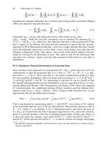
With respect to Equation 7.1, a common rule for finding the outlier region in a
single-step identifier is given by
out

α
n
,
ˆ
μ
n
,
ˆ
σ
2

n

=
{
x :
|
x −
ˆ
μ
n
|
> g(n,
α
n
)
ˆ
σ
n
}
, (7.2)
where n is the size of the sample;
ˆ
μ
n
and
ˆ
σ
n
are the estimated mean and standard
deviation of the target distribution based on the sample;

α
n
denotes the confidence
coefficient following the correction for multiple comparison tests; and g(n,
α
n
) de-
fines the limits (critical number of standard deviations) of the outlier regions.