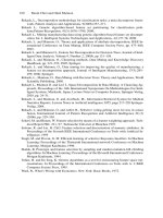
Data Mining and Knowledge Discovery Handbook, 2 Edition part 58 pot

550 Petr H
´
ajek
Brin, S., Motwani, R., and C. Silverstein. “Beyond market baskets: Generalizing association
rules to correlations”.
/>Chen, G., Wei, Q., and E. E. Kerre. “Fuzzy logic approaches for the mining of association
rules: an overview”. In: Data Mining and knowledge discovery approaches based on rule
induction techniques (Triantaphyllou E. et al., ed.) Kluwer, 2003
Dehaspe, L., and H. Toivonen. Discovery of frequent Datalog patterns. Data Mining and
knowledge discovery 1999; 3:7-36.
D
ˇ
zeroski, S., and N. Lavra
ˇ
c. Relational data mining. Springer, 2001
Ebbinghaus, H. D., Flum, J., and W. Thomas. Mathematical logic. Springer 1984.
Giudici, P. “Data Mining model comparison (Statistical models for Data Mining)”. Chapter
31.4.6, This volume.
Glymour, C., Madigan, D., Pregibon, D., and P. Smyth. “Statistical themes and lessons for
Data Mining.” Data Mining and knowledge discovery 1996; 1:25-42.
H
´
ajek, P. “The GUHA method and mining association rules.” Proc. CIMA’2001 (Bangor,
Wales) 533-539.
H
´
ajek, P. “The new version of the GUHA procedure ASSOC”, COMPSTAT 1984, 360-365.
H
´
ajek, P. “Generalized quantifiers, finite sets and Data Mining”. In: (Klopotek et al. ed.)
Intelligent Information Processing and Web Mining. Springer 2003, 489-496.

H
´
ajek, P., Havel, I. and M. Chytil. “The GUHA method of automatic hypotheses determina-
tion”, Computing 1966; 1:293-308.
H
´
ajek, P. and T. Havr
´
anek. Mechanizing Hypothesis Formation (Mathematical Foundations
for a General Theory), Springer-Verlag 1978, 396 pp.
H
´
ajek, P. and T. Havr
´
anek. Mechanizing Hypothesis Formation (Mathemati-
cal Foundations for a General Theory). Internet edition (freely accessible)
/>H
´
ajek, P. and M. Hole
ˇ
na. “Formal logics of discovery and hypotheses formation by ma-
chine”. Theor. Comp. Sci. 2003; 299:245-357.
H
´
ajek, P., Hole
ˇ
na, M. and J. Rauch. “The GUHA method and foundations of (relational)
data mining.” In: (de Swart et al., ed.) Theory and applications of relational structures as
knowledge instruments. Lecture Notes in Computer Science vol. 2929, Springer 2003,
17-37.

H
´
ajek, P., Sochorov
´
a, A. and J. Zv
´
arov
´
a. “GUHA for personal computers”, Comp. Stat. and
Data Anal. 1995; 19:149-153.
Hegland, M. “Data Mining techniques”. Acta numerica 2001; 10:313-355.
Hole
ˇ
na, M. “Exploratory data processing using a fuzzy generalization of the Guha ap-
proach”. In: J. F. Baldwin, editor, Fuzzy Logic, John Wiley and Sons, New York 1996,
213-229.
Hole
ˇ
na, M. “Fuzzy hypotheses for Guha implications”. Fuzzy Sets and Systems, 1998;
98:101–125.
Hole
ˇ
na, M. “A fuzzy logic framework for testing vague hypotheses with empirical data”.
In: Proceedings of the Fourth International ICSC Symposium on Soft Computing and
Intelligent Systems for Industry, ICSC Academic Press 2001, 401–407.
Hole
ˇ
na, M. “A fuzzy logic generalization of a Data Mining approach.” Neural Network
World 2001; 11:595–610.
Hole

ˇ
na, M. “Exploratory data processing using a fuzzy generalization of the GUHA ap-
proach”, Fuzzy Logic, Baldwin et al., ed. Willey et Sons New York 1996, 213-229.
H
¨
oppner, F. “Association rules”. Chapter 14.7.3, This volume.
26 Logics for Data Mining 551
Liu, W., Alvarez, S. A., and C. Ruiz. “Collaborative recommendation via adaptive association
rule mining”. KDD-2000 Workshop on Web Mining for E-Commerce, Boston, MA.
Rauch, J. “Logical problems of statistical data analysis in databases”. Proc. Eleventh Int.
Seminar on Database Management Systems 1988, 53-63.
Rauch, J. “GUHA as a Data Mining Tool, Practical Aspects of Knowledge management”.
Schweizer Informatiker Gesellshaft Basel 1996, 10 pp.
Rauch, J. “Logical Calculi for Knowledge Discovery”. Red. Komorowski, J. –
˙
Zytkow, J.,
Berlin, Springer Verlag 1997, 47-57.
Rauch, J.: Classes of Four-Fold Table Quantifiers. In Principles of Data Mining and Knowl-
edge Discovery, (J. Zytkow, M. Quafafou, eds.), Springer-Verlag, 203-211, 1998.
Rauch, J. “Four-fold Table Calculi and Missing Information”. In: JCIS’98 Proceedings, (Paul
P. Wang, editor), Association for Intelligent Machinery, 375-378.
Rauch, J., and M.
ˇ
Sim
˚
unek. “Mining for 4ft association rules”. Proc. Discovery Science 2000
Kyoto, Springer Verlag, 268-272.
Rauch, J. and M.
ˇ
Sim

˚
unek. “Mining for statistical association rules”. Proc. PAKDD 2001
Hong Kong, 149-158.
Rauch, J. “Association Rules and Mechanizing Hypothesis Formation”. Working notes of
ECML’2001 Workshop: Machine Learning as Experimental Philosophy of Science. See
also
ml/ecmlpkdd/.
Rauch, J. and M.
ˇ
Sim
˚
unek. “Mining for 4ft Association Rules by 4ft-Miner”. In: INAP 2001,
The Proceeding of the International Rule-Based Data Mining – in conjunction with INAP
2001, Tokyo.
Rauch, J. “Interesting Association Rules and Multi-relational Association Rules”. Communi-
cations of Institute of Information and Computing Machinery, Taiwan, 2002; 5, 2:77-82.
˙
Zytkow, J. M. and R. Zembowicz. “Contingency tables as the foundation for concepts, con-
cept hierarchies and rules: the 49er approach”. Fundamenta informaticae 1997; 30:383-
399.
GUHA+– project web site click Research, Software.
/>
27
Wavelet Methods in Data Mining
Tao Li
1
, Sheng Ma
2
, and Mitsunori Ogihara
3

1
School of Computer Science Florida International University
Miami, FL 33199

2
Machine Learning for Systems, IBM T.J. Watson Research Center
19 Skyline Drive, Hawthorne, NY 10532

3
Computer Science Department, University of Rochester
Rochester, NY 14627-0226

Summary. Recently there has been significant development in the use of wavelet methods in
various Data Mining processes. This article presents general overview of their applications in
Data Mining. It first presents a high-level data-mining framework in which the overall process
is divided into smaller components. It reviews applications of wavelets for each component.
It discusses the impact of wavelets on Data Mining research and outlines potential future
research directions and applications.
Key words:
Wavelet Transform, Data Management, Short Time Fourier Transform, Heisenberg’s
Uncertainty Principle, Discrete Wavelet Transform, Multiresolution Analysis, Harr Wavelet
Transform, Trend and Surprise Abstraction, Preprocessing, Denoising, Data Transformation,
Dimensionality Reduction, Distributed Data Mining
27.1 Introduction
The wavelet transform is a synthesis of ideas that emerged over many years from different
fields. Generally speaking, the wavelet transform is a tool that partitions data, functions, or
operators into different frequency components and then studies each component with a reso-
lution matched to its scale (Daubechies, 1992). Therefore, it can provide economical and in-
formative mathematical representation of many objects of interest (Abramovich et al., 2000).
Nowadays many software packages contain fast and efficient programs that perform wavelet

transforms. Due to such easy accessibility wavelets have quickly gained popularity among
scientists and engineers, both in theoretical research and in applications.
Data Mining is a process of automatically extracting novel, useful, and understandable
patterns from a large collection of data. Over the past decade this area has become significant
both in academia and in industry. Wavelet theory could naturally play an important role in Data
O. Maimon, L. Rokach (eds.), Data Mining and Knowledge Discovery Handbook, 2nd ed.,
DOI 10.1007/978-0-387-09823-4_27, © Springer Science+Business Media, LLC 2010
554 Tao Li, Sheng Ma, and Mitsunori Ogihara
Mining because wavelets could provide data presentations that enable efficient and accurate
mining process and they can also could be incorporated at the kernel for many algorithms.
Although standard wavelet applications are mainly on data with temporal/spatial localities
(e.g., time series data, stream data, and image data), wavelets have also been successfully
applied to various Data Mining domains.
In this chapter we present a general overview of wavelet methods in Data Mining with rel-
evant mathematical foundations and of research in wavelets applications. An interested reader
is encouraged to consult with other chapters for further reading (for references, see (Li, Li,
Zhu, and Ogihara, 2003)). This chapter is organized as follows: Section 27.2 presents a high-
level Data Mining framework, which reduces Data Mining process into four components. Sec-
tion 27.3 introduces some necessary mathematical background. Sections 27.4, 27.5, and 27.6
review wavelet applications in each of the components. Finally, Section 27.7 concludes.
27.2 A Framework for Data Mining Process
Here we view Data Mining as an iterative process consisting of: data management, data pre-
processing, core mining process and post-processing.Indata management, the mechanism
and structures for accessing and storing data are specified. The subsequent data preprocessing
is an important step, which ensures the data quality and improves the efficiency and ease of the
mining process. Real-world data tend to be incomplete, noisy, inconsistent, high dimensional
and multi-sensory etc. and hence are not directly suitable for mining. Data preprocessing
includes data cleaning to remove noise and outliers, data integration to integrate data from
multiple information sources, data reduction to reduce the dimensionality and complexity of
the data, and data transformation to convert the data into suitable forms for mining. Core min-

ing refers to the essential process where various algorithms are applied to perform the Data
Mining tasks. The discovered knowledge is refined and evaluated in post-processing stage.
The four-component framework above provides us with a simple systematic language for
understanding the steps that make up the data mining process. Of the four, post-processing
mainly concerns the non-technical work such as documentation and evaluation, we will focus
our attention on the first three components.
27.3 Wavelet Background
27.3.1 Basics of Wavelet in L
2
(R)
So, first, what is a wavelet? Simply speaking, a mother wavelet is a function
ψ
(x) such that
{
ψ
(2
j
x−k),i,k ∈Z}is an orthonormal basis of L
2
(R). The basis functions are usually referred
to wavelets
4
. The term wavelet means a small wave. The smallness refers to the condition that
we desire that the function is of finite length or compactly supported. The wave refers to the
condition that the function is oscillatory. The term mother implies that the functions with
different regions of support that are used in the transformation process are derived by dilation
and translation of the mother wavelet.
4
Note that this orthogonality is not an essential property of wavelets. We include it in the def-
inition because we discuss wavelet in the context of Daubechies wavelet and orthogonality

is a good property in many applications.
27 Wavelet Methods in Data Mining 555
At first glance, wavelet transforms are very much the same as Fourier transforms except
they have different bases. So why bother to have wavelets? What are the real differences
between them? The simple answer is that wavelet transform is capable of providing time
and frequency localizations simultaneously while Fourier transforms could only provide fre-
quency representations. Fourier transforms are designed for stationary signals because they
are expanded as sine and cosine waves which extend in time forever, if the representation
has a certain frequency content at one time, it will have the same content for all time. Hence
Fourier transform is not suitable for non-stationary signal where the signal has time varying
frequency (Polikar, 2005). Since FT doesn’t work for non-stationary signal, researchers have
developed a revised version of Fourier transform, The Short Time Fourier Transform (STFT).
In STFT, the signal is divided into small segments where the signal on each of these segments
could be assumed as stationary. Although STFT could provide a time-frequency representa-
tion of the signal, Heisenberg’s Uncertainty Principle makes the choice of the segment length
a big problem for STFT. The principle states that one cannot know the exact time-frequency
representation of a signal and one can only know the time intervals in which certain bands of
frequencies exist. So for STFT, longer length of the segments gives better frequency resolu-
tion and poorer time resolution while shorter segments lead to better time resolution but poorer
frequency resolution. Another serious problem with STFT is that there is no inverse, i.e., the
original signal can not be reconstructed from the time-frequency map or the spectrogram.
01
0
2
1
3
4
23
4
Time(seconds/T)

Frequency
Fig. 27.1. Time-Frequency Structure of
STFT. The graph shows that time and fre-
quency localizations are independent. The
cells are always square.
0
0
7
46
Time(seconds/T)
Frequency
2813 5 7
1
3
2
6
5
4
Fig. 27.2. Time Frequency structure of
WT. The graph shows that frequency res-
olution is good for low frequency and time
resolution is good at high frequencies.
Wavelet is designed to give good time resolution and poor frequency resolution at high
frequencies and good frequency resolution and poor time resolution at low frequencies (Po-
likar, 2005). This is useful for many practical signals since they usually have high frequency
components for a short durations (bursts) and low frequency components for long durations
(trends). The time-frequency cell structures for STFT and WT are shown in Figure 27.1 and
Figure 27.2 , respectively. In Data Mining practice, the key concept in use of wavelets is the
discrete wavelet transform (DWT). Our discussions will focus on DWT.
27.3.2 Dilation Equation

How to find the wavelets? The key idea is self-similarity. Start with a function
φ
(x) that
is made up of smaller version of itself. This is the refinement (or 2-scale, dilation) equation
φ
(x)=
∑
∞
k=−∞
a
k
φ
(2x−k), where a

k
s are called filter coefficients or masks. The function
φ
(x)
is called the scaling function (or father wavelet). Under certain conditions,
556 Tao Li, Sheng Ma, and Mitsunori Ogihara
ψ
(x)=
∞
∑
k=−∞
(−1)
k
b
k
φ

(2x −k)=
∞
∑
k=−∞
(−1)
k
¯a
1−k
φ
(2x −k) (27.1)
gives a wavelet
5
. Figure 27.3 shows Haar wavelet
6
and Figure 27.4 shows Daubechies-
2(db
2
) wavelet that is supported on intervals [0, 3]. In general, db
n
represents the family of
Daubechies Wavelets and n is the order. Generally it can be shown that: (1) The support for
db
n
is on the interval [0,2n−1], (2) The wavelet db
n
has n vanishing moments, and (3) The
regularity increases with the order. db
n
has rn continuous derivatives (r is about 0.2).
0 0.5 1 1.5

0
0.2
0.4
0.6
0.8
1
1.2
1.4
db1 : phi
0 0.5 1 1.5
−1.5
−1
−0.5
0
0.5
1
1.5
db1 : psi
Fig. 27.3. Haar Wavelet.
0 1 2 3 4
−0.4
−0.2
0
0.2
0.4
0.6
0.8
1
1.2
1.4

db2 : phi
0 1 2 3 4
−1.5
−1
−0.5
0
0.5
1
1.5
2
db2 : psi
Fig. 27.4. Daubechies-2(db
2
) Wavelet.
27.3.3 Multiresolution Analysis (MRA) and Fast DWT Algorithm
How to efficiently compute wavelet transforms? To answer the question, we need to touch
on some material of Multiresolution Analysis (MRA). MRA was first introduced in (Mal-
lat, 1989) and there is a fast family of algorithms based on it. The motivation of MRA is to
use a sequence of embedded subspaces to approximate L
2
(R) so that a proper subspace for
a specific application task can be chosen to get a balance between accuracy and efficiency.
Mathematically, MRA studies the property of a sequence of closed subspaces V
j
, j ∈Z which
approximate L
2
(R) and satisfy ···V
−2
⊂V

−1
⊂V
0
⊂V
1
⊂V
2
⊂···,

j∈Z
V
j
= L
2
(R) (L
2
(R)
space is the closure of the union of all V
j
), and

j∈Z
V
j
= /0 (the intersection of all V
j
is empty).
So what does multiresolution mean? The multiresolution is reflected by the additional re-
quirement f ∈V
j

⇐⇒ f (2x) ∈V
j+1
, j ∈Z (This is equivalent to f (x) ∈V
0
⇐⇒ f (2
j
x) ∈V
j
),
i.e., all the spaces are scaled versions of the central space V
0
.
So how does this related to wavelets? Because the scaling function
φ
easily generates a
sequence of subspaces which can provide a simple multiresolution analysis. First, the transla-
tions of
φ
(x), i.e.,
φ
(x −k),k ∈ Z, span a subspace, say V
0
(Actually,
φ
(x −k),k ∈ Z consti-
tutes an orthonormal basis of the subspace V
0
). Similarly 2
−1/2
φ

(2x −k),k ∈ Z span another
subspace, say V
1
. The dilation equation tells us that
φ
can be represented by a basis of V
1
.
It implies that
φ
falls into subspace V
1
and so the translations
φ
(x −k),k ∈ Z also fall into
subspace V
1
. Thus V
0
is embedded into V
1
. With different dyadic, it is straightforward to ob-
tain a sequence of embedded subspaces of L
2
(R) from only one function. It can be shown
that the closure of the union of these subspaces is exactly L
2
(R) and their intersections are
5
¯a means the conjugate of a.

6
Haar wavelet represents the same wavelet as Daubechies wavelets with support at [0,1],
called db
1
.
27 Wavelet Methods in Data Mining 557
empty sets (Daubechies, 1992). here, j controls the observation resolution while k controls the
observation location. Formal proof of wavelets’ spanning complement spaces can be found
in (Daubechies, 1992).
Layer 0
Layer 1
Layer 2
Layer 3
12 16 20
11 18 21
10
11
1
1012
12 10
=
=
+
-
( ) /
(
2
) / 2
Wavelet spac
e

Fig. 27.5. Fast Discrete Wavelet Transform.
A direct application of multiresolution analysis is the fast discrete wavelet transform algo-
rithm, called the pyramid algorithm (Mallat, 1989). The core idea is to progressively smooth
the data using an iterative procedure and keep the detail along the way, i.e., analyze projections
of f to W
j
. We use Haar wavelets to illustrate the idea through the following example. In Fig-
ure 27.5, the raw data is in resolution 3 (also called layer 3). After the first decomposition, the
data are divided into two parts: one is of average information (projection in the scaling space
V
2
and the other is of detail information (projection in the wavelet space W
2
). We then repeat
the similar decomposition on the data in V
2
, and get the projection data in V
1
and W
1
, etc. The
fact that L
2
(R) is decomposed into an infinite wavelet subspace is equivalent to the statement
that
ψ
j,k
, j,k ∈ Z span an orthonormal basis of L
2
(R). An arbitrary function f ∈ L

2
(R) then
can be expressed as f (x)=
∑
j,k∈Z
d
j,k
ψ
j,k
(x), where d
j,k
= f,
ψ
j,k
 is called the wavelet
coefficients. Note that j controls the observation resolution and k controls the observation lo-
cation. If data in some location are relatively smooth (it can be represented by low-degree
polynomials), then its corresponding wavelet coefficients will be fairly small by the vanishing
moment property of wavelets.
27.3.4 Illustrations of Harr Wavelet Transform
We demonstrate the Harr wavelet transform using a discrete time series x(t), where 0 ≤t ≤2
K
.
In L
2
(R), discrete wavelets can be represented as
φ
m
j
(t)=2

−j/2
φ
(2
−j
t −m), where j and
m are positive integers. j represents the dilation, which characterizes the function
φ
(t) at
different time-scales. m represents the translation in time. Because
φ
m
j
(t) are obtained by
dilating and translating a mother function
φ
(t), they have the same shape as the mother wavelet
and therefore self-similar to each other.
A discrete-time process x(t) can be represented through its inverse wavelet transform
x(t)=
∑
K
j=1
∑
2
K−j
−1
m=0
d
m
j

φ
m
j
(t)+
φ
0
, where 0 ≤t < 2
K
.
φ
0
is equal to the average value of x(t)
over t ∈ [0,2
K
−1]. Without loss of generality,
φ
0
is assumed to be zero. d
m
j
’s are wavelet
coefficients and can be obtained through the wavelet transform d
m
j
=
∑
2
K
−1
t=0

x(t)
φ
m
j
(t).Toex-
plore the relationships among wavelets, a tree diagram and the corresponding one-dimensional
558 Tao Li, Sheng Ma, and Mitsunori Ogihara
indices of wavelet coefficients were defined (Luettgen, 1993). The left picture of Figure 27.6
shows an example of Haar wavelets for K = 3, and the right figure shows the corresponding
tree diagram. The circled numbers represent the one-dimensional indices of the wavelet basis
functions, and are assigned sequentially to wavelet coefficients from the top to the bottom
down and the left to the right. The one-dimensional index s is thus a one-to-one mapping to
the two dimensional index ( j(s),m(s)), where j(s) and m(s) represent the scale and the shift
indices of the s-th wavelet. The equivalent notation
7
of d
s
is then d
m(s)
j(s)
. In addition, we denote
the parent and the neighboring wavelets of a wavelet through the tree diagram. As shown in
Figure 27.6,
γ
(s) and
ν
(s) are the parent and the left neighbor of node s, respectively.
27.3.5 Properties of Wavelets
In this section, we summarize and highlight the properties of wavelets which make they are
useful tools for Data Mining and many other applications.

4567
s
ν (s)
1
4
5
6
7
2
3
j=1
j=2
j=3
t
12345678
1
2
3
γ (s)
γ (s)
2
Fig. 27.6. Left figure shows the Haar wavelet basis functions. Right figure illustrates the
corresponding tree diagram and two types of operations. The number in the circle represents
the one dimension index of the wavelet basis functions. For example, the equivalent notation
of d
2
1
is d
6
. s,

ν
(s) and
γ
(s) represent the one dimension index of wavelet coefficients.
γ
(s) is
defined to be the parent node of node s.
ν
(s) is defined to be the left neighbor of node s.
Computational Complexity: First, the computation of wavelet transform can be very
efficient. Discrete Fourier transform(DFT) requires O(N
2
) multiplications and fast Fourier
transform also needs O(N logN) multiplications. However fast wavelet transform based on
Mallat’s pyramidal algorithm) only needs O(N) multiplications. The space complexity is also
linear.
Vanishing Moments: Another important property of wavelets is vanishing moments. A
function f (x) which is supported in bounded region
ω
is called to have n-vanishing moments if
it satisfies the following equation:

ω
f (x)x
j
dx = 0, j = 0,1, ,n. For example, Haar wavelet
has 1-vanishing moment and db
2
has 2-vanishing moment. The intuition of vanishing mo-
ments of wavelets is the oscillatory nature which can thought to be the characterization of

difference or details between a datum with the data in its neighborhood. Note that the filter
[1, -1] corresponding to Haar wavelet is exactly a difference operator. With higher vanishing
moments, if data can be represented by low-degree polynomials, their wavelet coefficients are
equal to zero.
Compact Support: Each wavelet basis function is supported on a finite interval. Compact
support guarantees the localization of wavelets. In other words, processing a region of data
with wavelet does not affect the the data out of this region.
7
For example, d
6
is d
2
1
(The shift index, m, starts from 0.) in the given example.
27 Wavelet Methods in Data Mining 559
Decorrelated Coefficients: Another important aspect of wavelets is their ability to reduce
temporal correlation so that the correlation of wavelet coefficients are much smaller than the
correlation of the corresponding temporal process (Flandrin, 1992). Hence, the wavelet trans-
form could be able used to reduce the complex process in the time domain into a much simpler
process in the wavelet domain.
Parseval’s Theorem: Assume that e ∈ L
2
and
ψ
i
be the orthonormal basis of L
2
. Parse-
val’s theorem states that e
2

2
=
∑
i
| < e,
ψ
i
> |
2
. In other words, the energy, which is defined
to be the square of its L
2
norm, is preserved under the orthonormal wavelet transform.
In addition, the multi-resolution property of scaling and wavelet functions leads to hi-
erarchical representations and manipulations of the objects and has widespread applications.
There are also some other favorable properties of wavelets such as the symmetry of scaling and
wavelet functions, smoothness and the availability of many different wavelet basis functions
etc.
27.4 Data Management
One of the features that distinguish Data Mining from other types of data analytic tasks is
the huge amount of data. The purpose of data management is to find methods for storing data
to facilitate fast and efficient access. The wavelet transformation provides a natural hierarchy
structure and multidimensional data representation and hence could be applied to data manage-
ment. A novel wavelet based tree structures was introduced in (Shahabi et al., 2001, Shahabi
et al., 2000): TSA-tree and 2D TSA-tree, to improve the efficiency of multilevel trends and
surprise queries on time sequence data. Frequent queries on time series data are to identify
rising and falling trends and abrupt changes at multiple level of abstractions. To support such
multi-level queries, a large amount of raw data usually needs to be retrieved and processed.
TSA (Trend and Surprise Abstraction) tree is designed to expedite the query process. It is
constructed based on the procedure of discrete wavelet transform. The root is the original time

series data. Each level of the tree corresponds to a step in wavelet decomposition. At the first
decomposition level, the original data is decomposed into a low frequency part (trend) and a
high frequency part (surprise). The left child of the root records the trend and the right child
records the surprise. At the second decomposition level, the low frequency part obtained in the
first level is further divided into a trend part and a surprise part. This process is repeated until
the last level of the decomposition. The structure of the TSA tree is described in Figure 27.7.
The 2D TSA tree is just the two dimensional extensions of the TSA tree using two dimensional
discrete wavelet transform.
27.5 Preprocessing
Real world data sets are usually not directly suitable for performing Data Mining algorithms.
They contain noise, missing values and may be inconsistent. In addition, real world data sets
tend to be too large and high-dimensional. Wavelets provide a way to estimate the underly-
ing function from the data. With the vanishing moment property of wavelets, we know that
only some wavelet coefficients are significant in most cases. By retaining selective wavelet
coefficients, wavelet transform could then be applied to denoising and dimensionality reduc-
tion. Moreover, since wavelet coefficients are generally decorrelated, we could transform the
original data into wavelet domain and then carry out Data Mining tasks.