Data Mining and Knowledge Discovery Handbook, 2 Edition part 109 pptx

1060
errors. While the algorithm is perhaps the most commonly used clustering algorithm in the
literature, one of its shortcomings is the fact that the number of clusters, K, must be pre-
specified.
Clustering has been used in many application domains including biology, medicine, an-
thropology, marketing, and economics. It is also a vital process for condensing and summariz-
ing information, since it can provide a synopsis of the stored data. Similar to query by content,
there are two types of time series clustering: whole clustering and subsequence clustering.
The notion of whole clustering is similar to that of conventional clustering of discrete objects.
Given a set of individual time series data, the objective is to group similar time series into the
same cluster. On the other hand, given a single (typically long) time series, subsequence clus-
tering is performed on each individual time series (subsequence) extracted from the long time
series with a sliding window. Subsequence clustering is a common pre-processing step for
many pattern discovery algorithms, of which the most well-known being the one proposed for
time series rule discovery. Recent empirical and theoretical results suggest that subsequence
clustering may not be meaningful on an entire dataset (Keogh et al., 2003), and that clustering
should only be applied to a subset of the data. Some feature extraction algorithm must choose
the subset of data, but we cannot use clustering as the feature extraction algorithm, as this
would open the possibility of a chicken and egg paradox. Several researchers have suggested
using time series motifs (see below) as the feature extraction algorithm (Chiu et al., 2003).
56.3.4 Prediction (Forecasting)
Prediction can be viewed as a type of clustering or classification. The difference is that pre-
diction is predicting a future state, rather than a current one. Its applications include obtain-
ing forewarning of natural disasters (flooding, hurricane, snowstorm, etc), epidemics, stock
crashes, etc. Many time series prediction applications can be seen in economic domains,
where a prediction algorithm typically involves regression analysis. It uses known values of
data to predict future values based on historical trends and statistics. For example, with the
rise of competitive energy markets, forecasting of electricity has become an essential part of
an efficient power system planning and operation. This includes predicting future electricity
demands based on historical data and other information, e.g. temperature, pricing, etc. As
another example, the sales volume of cellular phone accessories can be forecasted based on

the number of cellular phones sold in the past few months. Many techniques have been pro-
posed to increase the accuracy of time series forecast, including the use of neural network and
dimensionality reduction techniques.
56.3.5 Summarization
Since time series data can be massively long, a summarization of the data may be useful and
necessary. A statistic summarization of the data, such as the mean or other statistical prop-
erties can be easily computed even though it might not be particularly valuable or intuitive
information. Rather, we can often utilize natural language, visualization, or graphical sum-
marization to extract useful or meaningful information from the data. Anomaly detection and
motif discovery (see the next section below) are special cases of summarization where only
anomalous/repeating patterns are of interest and reported. Summarization can also be viewed
as a special type of clustering problem that maps data into subsets with associated simple
(text or graphical) descriptions and provides a higher-level view of the data. This new simpler
Chotirat Ann Ratanamahatana et al.
56 Mining Time Series Data 1061
description of the data is then used in place of the entire dataset. The summarization may be
done at multiple granularities and for different dimensions.
Some of popular approaches for visualizing massive time series datasets include Time-
Searcher, Calendar-Based Visualization, Spiral and VizTree.
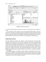
TimeSearcher (Hochheiser and Shneiderman, 2001) is a query-by-example time series
exploratory and visualization tool that allows user to retrieve time series by creating queries,
so called TimeBoxes. Figure 56.8 shows three TimeBoxes being drawn to specify time series
that start low, increase, then fall once more. However, some knowledge about the datasets
may be needed in advance and users need to have a general idea of what to look for or what is
interesting.
Fig. 56.8. The TimeSearcher visual query interface. A user can filter away sequences that are
not interesting by insisting that all sequences have at least one data point within the query
boxes
Cluster and Calendar-Based Visualization (Wijk and Selow, 1999) is a visualization sys-
tem that ‘chunks’ time series data into sequences of day patterns, and these day patterns are

clustered using a bottom-up clustering algorithm. The system displays patterns represented
by cluster average, along with a calendar with each day color-coded by the cluster it belongs
to. Figure 56.9 shows an example view of this visualization scheme. From viewing patterns
which are linked to a calendar we can potentially discover simple rules such as: “In the winter
months the power consumption is greater than in summer months”.
1062
Fig. 56.9. The cluster and calendar-based visualization on employee working hours data. It
shows six clusters, representing different working-day pattern
Spiral (Weber et al., 2000) maps each periodic section of time series onto one “ring”
and attributes such as color and line thickness are used to characterize the data values. The
main use of the approach is the identification of periodic structures in the data. Figure 56.10
displays the annual power usage that characterizes the normal “9-to-5” working week pattern.
However, the utility of this tool is limited for time series that do not exhibit periodic behaviors,
or when the period is unknown.
Fig. 56.10. The Spiral visualization approach applied to the power usage dataset
VizTree (Lin et al., 2004) is recently introduced with the aim to discover previously un-
known patterns with little or no knowledge about the data; it provides an overall visual sum-
mary, and potentially reveal hidden structures in the data. This approach first transforms the
Chotirat Ann Ratanamahatana et al.
56 Mining Time Series Data 1063
time series into a symbolic representation, and encodes the data in a modified suffix tree in
which the frequency and other properties of patterns are mapped onto colors and other visual
properties. Note that even though the tree structure needs the data to be discrete, the original
time series data is not. Using a time-series discretization introduced in (Lin et al., 2003), con-
tinuous data can be transformed into discrete domain, with certain desirable properties such as
lower-bounding distance, dimensionality reduction, etc. While frequently occurring patterns
can be detected by thick branches in VizTree, simple anomalous patterns can be detected by
unusually thin branches. Figure 56.11 demonstrates both motif discovery and simple anomaly
detection on ECG data.
Fig. 56.11. ECG data with anomaly is shown. While the subsequence tree can be used to

identify motifs, it can be used for simple anomaly detection as well
56.3.6 Anomaly Detection
In time series Data Mining and monitoring, the problem of detecting anomalous/surprising/novel
patterns has attracted much attention (Dasgupta and Forrest, 1999,Ma and Perkins, 2003,Sha-
habi et al., 2000). In contrast to subsequence matching, anomaly detection is identification of
previously unknown patterns. The problem is particularly difficult because what constitutes an
anomaly can greatly differ depending on the task at hand. In a general sense, an anomalous
behavior is one that deviates from “normal” behavior. While there have been numerous defi-
nitions given for anomalous or surprising behaviors, the one given by (Keogh et al., 2002) is
unique in that it requires no explicit formulation of what is anomalous. Instead, the authors
simply define an anomalous pattern as on “whose frequency of occurrences differs substan-
tially from that expected, given previously seen data”. The problem of anomaly detection in
time series has been generalized to include the detection of surprising or interesting patterns
(which are not necessarily anomalies). Anomaly detection is closely related to Summarization,
as discussed in the previous section. Figure 56.12 illustrates the idea.
1064
Fig. 56.12. An example of anomaly detection from the MIT-BIH Noise Stress Test Database.
Here, we show only a subsection containing the two most interesting events detected by the
compression-based algorithm (Keogh et al., 2004) (the thicker the line, the more interesting
the subsequence). The gray markers are independent annotations by a cardiologist indicating
Premature Ventricular Contractions.
56.3.7 Segmentation
Segmentation in time series is often referred to as a dimensionality reduction algorithm. Al-
though the segments created could be polynomials of an arbitrary degree, the most common
representation of the segments is of linear functions. Intuitively, a Piecewise Linear Represen-
tation (PLR) refers to the approximation of a time series Q, of length n, with K straight lines.
Figure 56.13 contains an example.
Fig. 56.13. An example of a time series segmentation with its piecewise linear representation
Because K is typically much smaller than n, this representation makes the storage, trans-
mission, and computation of the data more efficient.

Although appearing under different names and with slightly different implementation de-
tails, most time series segmentation algorithms can be grouped into one of the following three
categories.
• Sliding-Windows (SW): A segment is grown until it exceeds some error bound. The
process repeats with the next data point not included in the newly approximated segment.
• Top-Down (TD): The time series is recursively partitioned until some stopping criteria is
met.
• Bottom-Up (BU): Starting from the finest possible approximation, segments are merged
until some stopping criteria are met.
We can measure the quality of a segmentation algorithm in several ways, the most obvious
of which is to measure the reconstruction error for a fixed number of segments. The recon-
struction error is simply the Euclidean distance between the original data and the segmented
representation. While most work in this area has consider static cases, recently researchers
have consider obtaining and maintaining segmentations on streaming data sources (Palpanas
et al., 2004)
Chotirat Ann Ratanamahatana et al.
56 Mining Time Series Data 1065
56.4 Time Series Representations
As noted in the previous section, time series datasets are typically very large, for example,
just eight hours of electroencephalogram data can require in excess of a gigabyte of storage.
Rather than analyzing or finding statistical properties on time series data, time series data
miners’ goal is more towards discovering useful information from the massive amount of data
efficiently. This is a problem because for almost all Data Mining tasks, most of the execution
time spent by algorithm is used simply to move data from disk into main memory. This is
acknowledged as the major bottleneck in Data Mining because many na
¨
ıve algorithms require
multiple accesses of the data. As a simple example, imagine we are attempting to do k-means
clustering of a dataset that does not fit into main memory. In this case, every iteration of the
algorithm will require that data in main memory to be swapped. This will result in an algorithm

that is thousands of times slower than the main memory case.
With this in mind, a generic framework for time series Data Mining has emerged. The
basic idea (similar to GEMINI framework) can be summarized in Table 56.1.
Table 56.1. A generic time series Data Mining approach.
1) Create an approximation of the data, which will fit in main memory, yet retains
the essential features of interest.
2) Approximately solve the problem at hand in main memory.
3) Make (hopefully very few) accesses to the original data on disk to confirm
the solution obtained in Step 2, or to modify the solution so it agrees with the
solution we would have obtained on the original data.
As with most problems in computer science, the suitable choice of representation/approximation
greatly affects the ease and efficiency of time series Data Mining. It should be clear that the
utility of this framework depends heavily on the quality of the approximation created in Step
1). If the approximation is very faithful to the original data, then the solution obtained in main
memory is likely to be the same as, or very close to, the solution we would have obtained on the
original data. The handful of disk accesses made in Step 2) to confirm or slightly modify the
solution will be inconsequential, compared to the number of disks accesses required if we had
worked on the original data. With this in mind, there has been a huge interest in approximate
representation of time series, and various solutions to the diverse set of problems frequently
operate on high-level abstraction of the data, instead of the original data. This includes the
Discrete Fourier Transform (DFT) (Agrawal et al., 1993), the Discrete Wavelet Transform
(DWT) (Chan and Fu, 1999, Kahveci and Singh, 2001, Wu et al., 2000), Piecewise Linear,
and Piecewise Constant models (PAA) (Keogh et al., 2001, Yi and Faloutsos, 2000), Adaptive
Piecewise Constant Approximation (APCA) (Keogh et al., 2001), and Singular Value Decom-
position (SVD) (Kanth et al., 1998, Keogh et al., 2001, Korn et al., 1997).
Figure 56.14 illustrates a hierarchy of the representations proposed in the literature.
It may seem paradoxical that, after all the effort to collect and store the precise values of
a time series, the exact values are abandoned for some high level approximation. However,
there are two important reasons why this is so.
We are typically not interested in the exact values of each time series data point. Rather,

we are interested in the trends, shapes and patterns contained within the data. These may best
be captured in some appropriate high-level representation.
1066
Time Series
Representations
Data Adaptive Non Data Adaptive
SpectralWavelets
Piecewise
Aggregate
Approximation
Piecewise
Polynomial
Symbolic
Singula
r
Value
Decomposition
Random
Mappings
Piecewise
Linear
Approximation
Adaptive
Piecewise
Constant
Approximation
Discrete
Fourier
Transform
Discrete

Cosine
Transform
Haar
Daubechies
dbn n > 1
Coiflets Symlets
Sorted
Coefficients
Orthonormal Bi-Orthonormal
Interpretation Regression
Trees
Natural
Language
Strings
Fig. 56.14. A hierarchy of time series representations
As a practical matter, the size of the database may be much larger than we can effectively
deal with. In such instances, some transformation to a lower dimensionality representation of
the data may allow more efficient storage, transmission, visualization, and computation of the
data.
While it is clear no one representation can be superior for all tasks, the plethora of work on
mining time series has not produced any insight into how one should choose the best represen-
tation for the problem at hand and data of interest. Indeed the literature is not even consistent
on nomenclature. For example, one time series representation appears under the names Piece-
wise Flat Approximation (Faloutsos et al., 1997), Piecewise Constant Approximation (Keogh
et al., 2001) and Segmented Means (Yi and Faloutsos, 2000).
To develop the reader’s intuition about the various time series representations, we have
discussed and illustrated some of the well-known representations in the following subsections
below.
56.4.1 Discrete Fourier Transform
The first technique suggested for dimensionality reduction of time series was the Discrete

Fourier Transform (DFT) (Agrawal et al., 1993). The basic idea of spectral decomposition is
that any signal, no matter how complex, can be represented by the super position of a finite
number of sine/cosine waves, where each wave is represented by a single complex number
known as a Fourier coefficient. A time series represented in this way is said to be in the
frequency domain. A signal of length n can be decomposed into n/2 sine/cosine waves that
can be recombined into the original signal. However, many of the Fourier coefficients have
very low amplitude and thus contribute little to reconstructed signal. These low amplitude
coefficients can be discarded without much loss of information thereby saving storage space.
To perform the dimensionality reduction of a time series C of length n into a reduced
feature space of dimensionality N, the Discrete Fourier Transform of C is calculated. The
transformed vector of coefficients is truncated at N/2. The reason the truncation takes place
at N/2 and not at N is that each coefficient is a complex number, and therefore we need one
dimension each for the imaginary and real parts of the coefficients.
Given this technique to reduce the dimensionality of data from n to N, and the existence
of the lower bounding distance measure, we can simply “slot in” the DFT into the GEMINI
Chotirat Ann Ratanamahatana et al.
56 Mining Time Series Data 1067
Fig. 56.15. A visualization of the DFT dimensionality reduction technique
framework. The time taken to build the entire index depends on the length of the queries for
which the index is built. When the length is an integral power of two, an efficient algorithm
can be employed.
This approach, while initially appealing, does have several drawbacks. None of the imple-
mentations presented thus far can guarantee no false dismissals. Also, the user is required to
input several parameters, including the size of the alphabet, but it is not obvious how to choose
the best (or even reasonable) values for these parameters. Finally, none of the approaches sug-
gested will scale very well to massive data since they require clustering all data objects prior
to the discretizing step.
56.4.2 Discrete Wavelet Transform
Wavelets are mathematical functions that represent data or other functions in terms of the sum
and difference of a prototype function, so called the “analyzing” or “mother” wavelet. In this

sense, they are similar to DFT. However, one important difference is that wavelets are localized
in time, i.e. some of the wavelet coefficients represent small, local subsections of the data being
studied. This is in contrast to Fourier coefficients that always represent global contribution to
the data. This property is very useful for Multiresolution Analysis (MRA) of the data. The first
few coefficients contain an overall, coarse approximation of the data; addition coefficients can
be imagined as “zooming-in” to areas of high detail, as illustrated in Figure 56.16.
Fig. 56.16. A visualization of the DWT dimensionality reduction technique
Recently, there has been an explosion of interest in using wavelets for data compression,
filtering, analysis, and other areas where Fourier methods have previously been used. Chan
and Fu (1999) produced a breakthrough for time series indexing with wavelets by producing a
1068
distance measure defined on wavelet coefficients which provably satisfies the lower bounding
requirement. The work is based on a simple, but powerful type of wavelet known as the Haar
Wavelet. The Discrete Haar Wavelet Transform (DWT) can be calculated efficiently and an
entire dataset can be indexed in O(mn).
DTW does have some drawbacks, however. It is only defined for sequence whose length is
an integral power of two. Although much work has been undertaken on more flexible distance
measures using Haar wavelet (Huhtala et al., 1995,Struzik and Siebes, 1999), none of those
techniques are indexable.
56.4.3 Singular Value Decomposition
Singular Value Decomposition (SVD) has been successfully used for indexing images and
other multimedia objects (Kanth et al., 1998, Wu et al., 1996) and has been proposed for time
series indexing (Chan and Fu, 1999,Korn et al., 1997).
Singular Value Decomposition is similar to DFT and DWT in that it represents the shape
in terms of a linear combination of basis shapes, as shown in 56.17. However, SVD differs
from DFT and DWT in one very important aspect. SVD and DWT are local; they examine
one data object at a time and apply a transformation. These transformations are completely
independent of the rest of the data. In contrast, SVD is a global transformation. The entire
dataset is examined and is then rotated such that the first axis has the maximum possible
variance, the second axis has the maximum possible variance orthogonal to the first, the third

axis has the maximum possible variance orthogonal to the first two, etc. The global nature of
the transformation is both a weakness and strength from an indexing point of view.
Fig. 56.17. A visualization of the SVD dimensionality reduction technique.
SVD is the optimal transform in several senses, including the following: if we take the
SVD of some dataset, then attempt to reconstruct the data, SVD is the optimal (linear) trans-
form that minimizes reconstruction error (Ripley, 1996). Given this, we should expect SVD to
perform very well for the indexing task.
56.4.4 Piecewise Linear Approximation
The idea of using piecewise linear segments to approximate time series dates back to 1970s
(Pavlidis and Horowitz, 1974). This representation has numerous advantages, including data
Chotirat Ann Ratanamahatana et al.
56 Mining Time Series Data 1069
compression and noise filtering. There are numerous algorithms available for segmenting time
series, many of which were pioneered by (Pavlidis and Horowitz, 1974). Figure 56.18 shows
an example of a time series represented by piecewise linear segments.
Fig. 56.18. A visualization of the PLA dimensionality reduction technique
An open question is how to best choose K, the “optimal” number of segments used to
represent a particular time series. This problem involves a trade-off between accuracy and
compactness, and clearly has no general solution.
56.4.5 Piecewise Aggregate Approximation
The recent work (Keogh et al., 2001,Yi and Faloutsos, 2000) (independently) suggest approx-
imating a time series by dividing it into equal-length segments and recording the mean value
of the data points that fall within the segment. The authors use different names for this repre-
sentation. For clarity here, we refer to it as Piecewise Aggregate Approximation (PAA). This
representation reduces the data from n dimensions to N dimensions by dividing the time series
into N equi-sized ‘frames’. The mean value of the data falling within a frame is calculated,
and a vector of these values becomes the data reduced representation. When N = n, the trans-
formed representation is identical to the original representation. When N = 1, the transformed
representation is simply the mean of the original sequence. More generally, the transforma-
tion produces a piecewise constant approximation of the original sequence, hence the name,

Piecewise Aggregate Approximation (PAA). This representation is also capable of handling
queries of variable lengths.
In order to facilitate comparison of PAA with other dimensionality reduction techniques
discussed earlier, it is useful to visualize it as approximating a sequence with a linear combi-
nation of box functions. Figure 56.19 illustrates this idea.
This simple technique is surprisingly competitive with the more sophisticated transform.
In addition, the fact that each segment in PAA is of the same length facilitates indexing of this
representation.
56.4.6 Adaptive Piecewise Constant Approximation
As an extension to the PAA representation, Adaptive Piecewise Constant Approximation
(APCA) is introduced (Keogh et al., 2001). This representation allows the segments to have
arbitrary lengths, which in turn needs two numbers per segment. The first number records the