DISCRETE-SIGNAL ANALYSIS AND DESIGN- P6 pdf
Bạn đang xem bản rút gọn của tài liệu. Xem và tải ngay bản đầy đủ của tài liệu tại đây (148.1 KB, 5 trang )
FIRST PRINCIPLES 11
0
N−1
N
N/2
0
N/2
N−1
N
(a)
(b)
−4 −3 −2 −10+1 +2 +3
0
+1 +2 +3 +4 +5
−4 −3 −2 −1
+6 +7
N/2
0
(c)
(
d
)
1234567
N/2 − 1 N/2 + 1
N − 1
N = 8
Figure 1-1 InÞnite sequence operations for wave analysis. (a) The
segment of inÞnite periodic sequence from 0 to N −1. The next sequence
starts at N . (b) The Segment of inÞnite sequence from 0 to N −1 is not
periodic with respect to the rest of the inÞnite sequence. (c) The two-sided
sequence starts at −4 or 0. (d) The sequence starts at 0.
12 DISCRETE-SIGNAL ANALYSIS AND DESIGN
identiÞed in both time and amplitude. If the sequence is nonrepeating
(random), or if it is inÞnite in length, or if it is periodic but the sequence
is not chosen to be exactly one period, then this segment is not one
period of a truly periodic process, as shown in Fig. 1-1b. However, the
wave analysis math assumes that the part of the wave that is selected is
actually periodic within an inÞnite sequence, similar to Fig. 1-1a. The
selected sequence can then perhaps be referred to as “pseudo-periodic”,
and the analysis results are correct for that sequence. For example, the
entire sequence of Fig. 1-1b, or any segment of it, can be analyzed exactly
as though the selected segment is one period of an inÞnite periodic wave.
The results of the analysis are usually different for each different segment
that is chosen. If the 0 to N −1 sequence in Fig. 1-1b is chosen, the
analysis results are identical to the results for 0 to N −1 in Fig. 1-1a.
When selecting a segment of the data, for instance experimentally
acquired values, it is important to be sure that the selected data contains
the amount of information that is needed to get a sufÞciently accurate
analysis. If amplitude values change signiÞcantly between samples, we
must use samples that are more closely spaced. There is more about this
later in this chapter.
It is important to point out a fact about the time sequences x(n)in
Fig. 1-1. Although the samples are shown as thin lines that have very
little area, each line does represent a deÞnite amount of energy. The sum
of these energies, within a unit time interval, and if there are enough of
them so that the waveform is adequately represented (the Nyquist and
Shannon requirements) [Stanley, 1984, p. 49], contains very nearly the
same energy per unit time interval; in other words very nearly the same
average power (theoretically, exactly the same), as the continuous line
that is drawn through the tips of the samples [Carlson, 1986, pp. 351 and
624]. Another way to look at it is to consider a single sample at time (n)
and the distance from that sample to the next sample, at time (n +1). The
area of that rectangle (or trapezoid) represents a certain value of energy.
The value of this energy is proportional to the length (amplitude) of the
sample. We can also think of each line as a Dirac “impulse” that has zero
width but a deÞnite area and an amplitude x(n) that is a measure of its
energy. Its Laplace transform is equal to 1.0 times x (n).
If the signal has some randomness (nearly all real-world signals do),
the conclusion of adequate sampling has to be qualiÞed. We will see in
FIRST PRINCIPLES 13
later chapters, especially Chapter 6, that one record length (N )ofsucha
signal may not be adequate, and we must do an averaging operation, or
other more elaborate operations, on many such records.
Discrete sequences can also represent samples in the frequency domain,
and the same rules apply. The power in the adequate set of individual
frequencies over some speciÞed bandwidth is almost (or exactly) the same
as the power in the continuous spectrum within the same bandwidth, again
assuming adequate samples.
In some cases it will be more desirable, from a visual standpoint, to
work with the continuous curves, with this background information in
mind. Figure 1-6 is an example, and the discrete methods just mentioned
are assumed to be still valid.
TWO-SIDED TIME AND FREQUENCY
An important aspect of a periodic time sequence concerns the relative
time of occurrence. In Fig. 1-1a and b, the “present” item is located
at n =0. This is the reference point for the sequence. Items to the left
are “previous” and items to the right are “future”. Figure 1-1c shows an
8-point sequence that occurs between −4and+3. The “present” symbol
is at n =0, previous symbols are from −4to−1, and future symbols are
from +1to+3. In Fig. 1-1d the same sequence is shown labeled from 0
to +7. But the +4to+7 values are observed to have the same amplitudes
as the −4to−1 values in Fig. 1-1c. Therefore, the +4to+7 values of
Fig. 1-1d should be thought of as “previous” and they may be relabeled as
shown in Fig. 1-1d. We will use this convention consistently throughout
the book. Note that one location, N /2, is labeled both as +4and−4. This
location is special and will be important in later work. In computerized
waveform analysis and design, it is a good practice to use n =0asa
starting point for the sequence(s) to be processed, as in Fig. 1-1d, because
a possible source of confusion is eliminated.
A similar but slightly different idea occurs in the frequency-domain
sequence, which is usually a two-sided spectrum consisting of positive-
and negative-frequency harmonics, to be discussed in detail later. For
example, if Fig. 1-1c and d are frequency values X (k ), then −4to−1in
Fig. 1-1c and +4to+7 in Fig. 1-1d are negative frequencies. The value at
14 DISCRETE-SIGNAL ANALYSIS AND DESIGN
k =0 is the dc component, k =±1isthe±fundamental frequency, and
other ±k values are ±harmonics of the k =±1 value. The frequency
k =±N /2 is special, as discussed later. Because of the assumed steady-
state periodicity of the sequences, the Discrete Fourier Transform, often
correctly referred to in this book as the Discrete Fourier Series, and its
inverse transform are used to travel very easily between the time and
frequency domains.
An important thing to keep in mind is that in all cases, in this chapter or
any other where we perform a summation () from 0 to N −1, we assume
that all of the signiÞcant signal and noise energy that we are concerned
with lies within those boundaries. We are thus relieved of the integrations
from −∞ to +∞ that we Þnd in many textbooks, and life becomes sim-
pler in the discrete 0 to N −1 world. It also validates our assumptions
about the steady-state repetition of sequences. In Chapters 3 and 4 we look
at aliasing, spectral leakage, smoothing, and windowing, and these help to
assure our reliance on 0 to N −1. We can also increase N by 2
M
(M =2,
3, 4, ) as needed to encompass more time or more spectrum.
DISCRETE FOURIER TRANSFORM (SERIES)
A typical example of discrete-time x (n) values is shown in Fig. 1-2a. It
consists of 64 equally spaced real-valued samples 0 ≤n ≤63 of a sine
wave, peak amplitude A =1.0 V, to which a dc bias of Vdc =+1.0 V
has been added. Point n =N =64 is the beginning of the next sine wave
plus dc bias. The sequence x(n), including the dc component, is
x(n) = A sin
2π
n
N
K
x
+ Vdc volts (1-1)
where K
x
is the number of cycles per sequence length: in this example,
1.0. To Þnd the frequency spectrum X (k) for this x(n) sequence (Fig.
1-2b), we use the DFT of Eq. (1-2) [Oppenheim et al., 1983, p. 321]:
X(k) =
1
N
N−1
n=0
x(n) e
−j 2π
n
N
·k
volts, k = 0toN − 1 (1-2)
FIRST PRINCIPLES 15
−j 0.5
+j 0.5
k = 1
dc = +1.0
k = 0
k = 63
0
63
0
(a)
(b)
(c)
63
0 to N/2 − 1 = 32 freqs N/2 to N − 1 = 32 freqs
N = 64
0 to N = 64 freq intervals
0 to N −1 = 64 freq values, including dc
N/2 − 1 N/2
Figure 1-2 Sequence (a) is converted to a spectrum (b) and recon-
verted to a sequence (c). (a) 64-point sequence, sine wave plus dc bias.
(b) Two-sided spectrum of w to count freq part (a) showing ho values
and frequency intervals. (c) The spectrum of part (b) is reconverted to the
time sequence of part (a).
In this equation, for each discrete value of (k) from 0 to N −1, the func-
tion x (n) is multiplied by the complex exponential, whose magnitude =
1.0. Also, at each (n) a constant negative (clockwise) phase lag incre-
ment (−2πnk /N ) radians is added to the exponential. Figure 1-2b shows
that the spectrum has just two lines of amplitude ±j 0.5 at k =1 and 63,
which is correct for a sine wave of frequency 1.0, plus the dc at k =0.
These two lines combine coherently to produce a real sine wave of
amplitude A =1.0. The peak power in a 1.0 ohm resistor is not the sum of
the peak powers of the two components, which is (0.5
2
+0.5
2
) =0.5 W;
instead, the peak power is the square of the sum of the two components,
which is (0.5 +0.5)
2
=1.0 W. If the spectrum component X (k)hasareal