How to Display Data- P16 ppsx
Bạn đang xem bản rút gọn của tài liệu. Xem và tải ngay bản đầy đủ của tài liệu tại đây (166.88 KB, 5 trang )
Reporting study results 67
outcome, and it is said to have four cells (2 ϫ 2) (see also Chapter 3). The
most appropriate comparative summary measure for these data is the dif-
ference in proportions healed between the two groups.
The important contrast is between the 20% healed in the intervention
group compared to 16% in the control group. Since English script reads
naturally from left to right, it is recommended that the data for treatment
groups is in the columns in order that differences between groups can be
compared side by side as shown in Table 7.1.
Another advantage of the format in Table 7.1 is that with several out-
comes we can place the data for the different outcomes underneath each
other in separate rows. For example, Table 7.2 shows the ulcer healing rates
at 3 and 12 months. This format, with the groups in the columns, is also
Table 7.1 Cross-tabulation of treatment group (in
columns) vs. outcome (in rows) ulcer healed or not
healed at 12 weeks (n ϭ 206)
1
Group
Intervention Control
% (n ϭ 106) % (n ϭ 100)
Outcome
Healed 20% (21) 16% (16)
Not healed 80% (85) 84% (84)
Table 7.2 Ulcer healing rates at 3 and 12 months follow-up by treatment
group (maximum n ϭ 206)
1
Group Difference in P-value
b
Relaive
percentages
a
Risk
c
Intervention Control (95% CI) (95% CI)
Outcome
Healed at 3 20% 16% 4% 0.47 1.25
months (21/106) (16/100) (Ϫ7 to 14) (0.69–2.23)
Healed at 12 52% 42% 10% 0.20 1.24
months (42/81) (33/79) (Ϫ5 to 25) (0.89–1.73)
CI: Confi dence interval.
a
A positive difference indicates that the intervention group does better than the
control group.
b
P-values from chi-squared test.
c
A relative risk Ͼ 1 indicates that the intervention group does better than the control
group.
68 How to Display Data
favoured by leading medical journals, such as the British Medical Journal.
Note that no decimal places are reported for the percentages of ulcers
hea led or the difference, which makes the table clearer. The denominator
is presented for all the outcomes and thus it is clear that the sample size is
lower for the 12-month comparison. Also presented is a column with the
absolute difference in ulcer healing rates between the two groups, its 95%
confi dence interval and the P-value associated with this comparison. It is
recommended that when presenting confi dence intervals the word ‘to’ is
used to link the lower and upper limits rather than a dash symbol ‘–’ as it
can sometimes be diffi cult to know whether the upper limit is negative or
not if the dash symbol is used. When presenting a P-value it is important to
make clear what statistical test was used to derive it. In Table 7.2 the P-value
has come from the chi-squared test.
For two groups with a binary outcome there are several other ways of
comparing the groups, not just a comparison of two proportions. Alter-
natives include: the relative risk (RR); odds ratio (OR) and number needed
to treat (NNT). See Campbell et al. (2007) for more details on how to calcu-
late these summary measures.
2
The last column of data in Table 7.2 shows
the RR of an ulcer healing in the intervention group compared to an ulcer
healing in the control group, together with its 95% confi dence interval.
When there are more than two categories for the outcome variable, such
as a fi ve point symptom score scale (much better, better, same, worse, much
worse), these may also be incorporated in a format similar to Table 7.2, with
a separate line for each category of the variable. If the categories have a nat-
ural ordering such as the pain scale above, then this ordering should be pre-
served. If however, there is no natural ordering then the categories should
be ordered by size.
7.3 Tabulating the results of logistic regression analysis
The previous section in this chapter described a method for displaying
categorical outcome data. In addition to the grouping variable it is often
important to adjust for other explanatory variables, in which case a logistic
regression is usually carried out. One of the outcomes from the leg ulcer
study was ulcer status at 12 weeks (healed/not healed) and the results of a
logistic regression to assess the impact of various explanatory variables on
ulcer state at 12 weeks is presented in Table 7.3. When reporting the results
of a logistic regression analysis, as a minimum the estimated OR for the
regression coeffi cients, their confi dence intervals and associated P-values
should be presented. The sample size that the regression was based upon
should also be reported. If space allows, the regression coeffi cient and its
Reporting study results 69
standard error (SE) can also be reported, but as this is on a logarithmic
scale, it is not as helpful as the estimated OR. For logistic regression it is also
helpful to give some information about the goodness of fi t of the model to
the data. The simplest statistic for doing this is the Hosmer and Lemeshow
chi-squared statistics and we would recommend this is reported together
with the degrees of freedom and P-value so that the reader can judge
whether or not the model adequately fi ts the data.
3
7.4 Tabulating quantitative outcomes
In addition to displaying categorical outcomes, outcome data may be quan-
titative, either count or continuous. As part of a RCT comparing traditional
acupuncture with usual care for non-specifi c low back pain, HRQoL was
measured at 12 months, using the SF-36.
4
These data are shown in Table
7.4. Data for the two treatment groups is arranged in the columns and the
rows correspond to the eight SF-36 dimensions, and are ordered by mean
difference. The mean dimension scores (and their variability) are described
separately for each group. A 95% confi dence interval for the treatment
effect, (difference in mean scores), is reported. Exact P-values are reported
to two signifi cant fi gures in the last column of the table. A footnote to
the table is included describing how the SF-36 is scaled and scored, what
hypothesis test has been performed and how the treatment effect (mean dif-
ference) should be interpreted. Since the SF-36 is scored on a 0–100 scale
Table 7.3 Estimated OR from the multiple logistic regression model to predict ulcer
status (healed or not healed) at 12 weeks from baseline ulcer area, gender, marital
status and treatment group in 187 patients with venous leg ulcers
1
OR (95% CI) P-value
Intercept 0.15 0.003
Baseline ulcer area (cm
2
) 0.89 (0.82 to 0.96) 0.004
Gender (0 ϭ male, 1 ϭ female) 3.37 (1.21 to 9.34) 0.020
Marital status 0.670
Married (reference category) 1.00
Single (relative to married) 1.83 (0.47 to 7.19) 0.384
Divorced (relative to married) 0.49 (0.05 to 4.81) 0.543
Widowed (relative to married) 0.84 (0.35 to 2.00) 0.695
Group (0 ϭ Control, 1 ϭ Intervention) 1.80 (0.79 to 4.09) 0.159
CI: Confi dence interval.
Hosmer and Lemeshow test, χ
2
ϭ 11.22 on 8 degrees of freedom, P ϭ 0.19.
Y variable: Ulcer healed at 12 weeks (0 ϭ No, 1 ϭ Yes).
70 How to Display Data
Table 7.4 Mean SF-36 dimension scores at 12 months by treatment group
4
Treatment group
SF-36 Usual care Acupuncture Mean difference
b
dimension
a
n Mean (SD) n Mean (SD) (95% CI) P-value
c
Pain 68 58.3 (22.2) 147 64.0 (25.6) 5.7 0.12
(Ϫ1.4 to 12.8)
Role- 57 61.8 (42.8) 134 66.0 (40.0) 4.2 0.52
physical (Ϫ8.5 to 17.0)
Role- 57 78.4 (35.9) 133 78.2 (35.3) Ϫ0.2 0.98
emotional (Ϫ11.2 to 10.9)
General 56 65.4 (19.3) 134 64.8 (21.8) Ϫ0.6 0.87
health (Ϫ7.2 to 6.1)
Physical 57 73.4 (20.9) 133 71.7 (25.8) Ϫ1.7 0.65
functioning (Ϫ9.4 to 5.9)
Vitality 56 57.0 (21.6) 135 54.1 (23.3) Ϫ2.9 0.43
(Ϫ10.0 to 4.3)
Social 68 80.7 (22.1) 147 77.8 (25.2) Ϫ2.9 0.41
functioning (Ϫ10.0 to 4.1)
Mental 56 73.3 (15.4) 135 69.0 (20.4) Ϫ4.3 0.15
health (Ϫ10.3 to 1.6)
CI: Confi dence interval.
a
The SF-36 dimensions are scored on a 0 (poor) to 100 (good health) scale.
b
A positive mean difference indicates the acupuncture group has the better HRQoL.
c
P-value from two independent samples t-test.
these data are reported to a precision of one decimal place. Note that as the
number of observations varies considerably across the eight dimensions a
second table could also be produced for those individuals who had data on
all dimensions.
7.5 Plots for displaying outcome data
A useful plot for displaying continuous outcome data, when there are mul-
tiple variables all measured on the same scale, such as for the HRQoL data
in Table 7.4 is the spider or radar plot. Figure 7.1 shows a radar plot for the
mean SF-36 dimension scores, at 12 months follow-up, by treatment group
for the data presented in Table 7.4. The radar plot has eight spokes corre-
sponding to the eight dimensions of the SF-36, with the centre point of the
plot indicating a score of 0. It is clear from this plot that the two treatments
groups have similar mean HRQoL for all eight dimensions of the SF-36,
although Figure 7.1 conceals the fact that the sample size for each dimension
Reporting study results 71
varies considerably. We could report the number of subjects for each out-
come, but this would make the chart look rather messy. An alternative strat-
egy would be redraw the plot but including only those subjects who had
data for all outcomes.
The radar plot of Figure 7.1 clearly displays the mean SF-36 dimen-
sion scores by treatment group. However, for comparison purposes, what
is required is the contrast or difference in outcomes between the groups
and the associated uncertainty or confi dence interval around this esti-
mated treatment effect. These can be shown graphically using a forest plot
similar to those used for displaying the results of meta-analyses and system-
atic reviews, described later in this chapter. Figure 7.2 shows a forest plot
of the estimated treatment effect (mean difference in SF-36 scores between
the acupuncture and usual care groups) and the corresponding confi dence
interval, at 12 months, for the eight dimensions of the SF-36.
4
Figure 7.2 is visually impressive and the lack of any treatment effect for
HRQoL is readily apparent. Also note that the numbers used for each com-
parison are clearly displayed. This chart can be particularly useful in con-
ference presentations when much information needs to be conveyed to the
audience in a limited amount of time. However, much of the data presented
Figure 7.1 Radar or spider plot with mean scores, at 12 months follow-up, for the
eight dimensions of the SF-36 by treatment group, Note that the SF-36 dimensions
are scored on a 0 (poor) to 100 (good) health scale.
4
Physical function
General health
Role-emotional
Role-physical
Pain
100
50
0
Mental health
Social function
Vitality
Usual care (min n ϭ 56)
Acu
p
uncture (min n ϭ 133)