Econometric theory and methods, Russell Davidson - Chapter 4 ppt

Bạn đang xem bản rút gọn của tài liệu. Xem và tải ngay bản đầy đủ của tài liệu tại đây (439.71 KB, 54 trang )

Chapter 4
Hypothesis Testing in
Linear Regression Models
4.1 Introduction
As we saw in Chapter 3, the vector of OLS parameter estimates
ˆ
β is a random
vector. Since it would be an astonishing coincidence if
ˆ
β were equal to the
true parameter vector β
0
in any ﬁnite sample, we must take the randomness
of
ˆ
β into account if we are to make inferences about β. In classical economet-
rics, the two principal ways of doing this are p erforming hypothesis tests and
constructing conﬁdence intervals or, more generally, conﬁdence regions. We
will discuss the ﬁrst of these topics in this chapter, as the title implies, and the
second in the next chapter. Hypothesis testing is easier to understand than
the construction of conﬁdence intervals, and it plays a larger role in applied
econometrics.
In the next section, we develop the fundamental ideas of hypothesis testing
in the context of a very simple special case. Then, in Section 4.3, we review
some of the properties of several distributions which are related to the nor-
mal distribution and are commonly encountered in the context of hypothesis
testing. We will need this material for Section 4.4, in which we develop a
number of results about hypothesis tests in the classical normal linear model.
In Section 4.5, we relax some of the assumptions of that model and introduce
large-sample tests. An alternative approach to testing under relatively weak
assumptions is bootstrap testing, which we introduce in Section 4.6. Finally,

in Section 4.7, we discuss what determines the ability of a test to reject a
hypothesis that is false.
4.2 Basic Ideas
The very simplest sort of hypothesis test concerns the (population) mean from
which a random sample has been drawn. To test such a hypothesis, we may
assume that the data are generated by the regression model
y
t
= β + u
t
, u
t
∼ IID(0, σ
2
), (4.01)
Copyright
c
 1999, Russell Davidson and James G. MacKinnon 123
124 Hypothesis Testing in Linear Regression Models
where y
t
is an observation on the dependent variable, β is the population
mean, which is the only parameter of the regression function, and σ
2
is the
variance of the error term u
t
. The least squares estimator of β and its variance,
for a sample of size n, are given by
ˆ

β =
1
−
n
n

t=1
y
t
and Var (
ˆ
β) =
1
−
n
σ
2
. (4.02)
These formulas can either be obtained from ﬁrst principles or as special cases
of the general results for OLS estimation. In this case, X is just an n vector
of 1s. Thus, for the model (4.01), the standard formulas
ˆ
β = (X

X)
−1
X

y
and Var(

ˆ
β) = σ
2
(X

X)
−1
yield the two formulas given in (4.02).
Now suppose that we wish to test the hypothesis that β = β
0
, where β
0
is
some speciﬁed value of β.
1
The hypothesis that we are testing is called the
null hypothesis. It is often given the label H
0
for short. In order to test H
0
,
we must calculate a test statistic, which is a random variable that has a known
distribution when the null hypothesis is true and some other distribution when
the null hypothesis is false. If the value of this test statistic is one that might
frequently be encountered by chance under the null hypothesis, then the test
provides no evidence against the null. On the other hand, if the value of the
test statistic is an extreme one that would rarely be encountered by chance
under the null, then the test does provide evidence against the null. If this
evidence is suﬃciently convincing, we may decide to reject the null hypothesis
that β = β

0
.
For the moment, we will restrict the model (4.01) by making two very strong
assumptions. The ﬁrst is that u
t
is normally distributed, and the second
is that σ is known. Under these assumptions, a test of the hypothesis that
β = β
0
can b e based on the test statistic
z =
ˆ
β − β
0

Var(
ˆ
β)

1/2
=
n
1/2
σ
(
ˆ
β − β
0
). (4.03)
It turns out that, under the null hypothesis, z must be distributed as N(0, 1).

It must have mean 0 because
ˆ
β is an unbiased estimator of β, and β = β
0
under the null. It must have variance unity because, by (4.02),
E(z
2
) =
n
σ
2
E

(
ˆ
β − β
0
)
2

=
n
σ
2
σ
2
n
= 1.
1
It may be slightly confusing that a 0 subscript is used here to denote the value

of a parameter under the null hypothesis as well as its true value. So long
as it is assumed that the null hypothesis is true, however, there should b e no
possible confusion.
Copyright
c
 1999, Russell Davidson and James G. MacKinnon
4.2 Basic Ideas 125
Finally, to see that z must be normally distributed, note that
ˆ
β is just the
average of the y
t
, each of which must be normally distributed if the corre-
sponding u
t
is; see Exercise 1.7. As we will see in the next section, this
implies that z is also normally distributed. Thus z has the ﬁrst property that
we would like a test statistic to possess: It has a known distribution under
the null hypothesis.
For every null hypothesis there is, at least implicitly, an alternative hypothesis,
which is often given the lab el H
1
. The alternative hypothesis is what we are
testing the null against, in this case the model (4.01) with β = β
0
. Just as
important as the fact that z follows the N(0, 1) distribution under the null is
the fact that z do es not follow this distribution under the alternative. Suppose
that β takes on some other value, say β
1

. Then it is clear that
ˆ
β = β
1
+ ˆγ,
where ˆγ has mean 0 and variance σ
2
/n; recall equation (3.05). In fact, ˆγ
is normal under our assumption that the u
t
are normal, just like
ˆ
β, and so
ˆγ ∼ N(0, σ
2
/n). It follows that z is also normal (see Exercise 1.7 again), and
we ﬁnd from (4.03) that
z ∼ N(λ, 1), with λ =
n
1/2
σ
(β
1
− β
0
). (4.04)
Therefore, provided n is suﬃciently large, we would expect the mean of z to
be large and positive if β
1
> β

0
and large and negative if β
1
< β
0
. Thus we
will reject the null hypothesis whenever z is suﬃciently far from 0. Just how
we can decide what “suﬃciently far” means will be discussed shortly.
Since we want to test the null that β = β
0
against the alternative that β = β
0
,
we must perform a two-tailed test and reject the null whenever the absolute
value of z is suﬃciently large. If instead we were interested in testing the
null hypothesis that β ≤ β
0
against the alternative that β > β
0
, we would
perform a one-tailed test and reject the null whenever z was suﬃciently large
and positive. In general, tests of equality restrictions are two-tailed tests, and
tests of inequality restrictions are one-tailed tests.
Since z is a random variable that can, in principle, take on any value on the
real line, no value of z is absolutely incompatible with the null hypothesis,
and so we can never be absolutely certain that the null hypothesis is false.
One way to deal with this situation is to decide in advance on a rejection rule,
according to which we will choose to reject the null hypothesis if and only if
the value of z falls into the rejection region of the rule. For two-tailed tests,
the appropriate rejection region is the union of two sets, one containing all

values of z greater than some positive value, the other all values of z less than
some negative value. For a one-tailed test, the rejection region would consist
of just one set, containing either suﬃciently positive or suﬃciently negative
values of z, according to the sign of the inequality we wish to test.
A test statistic combined with a rejection rule is sometimes called simply a
test. If the test incorrectly leads us to reject a null hypothesis that is true,
Copyright
c
 1999, Russell Davidson and James G. MacKinnon
126 Hypothesis Testing in Linear Regression Models
we are said to make a Type I error. The probability of making such an error
is, by construction, the probability, under the null hypothesis, that z falls
into the rejection region. This probability is sometimes called the level of
signiﬁcance, or just the level, of the test. A common notation for this is α.
Like all probabilities, α is a number between 0 and 1, although, in practice, it
is generally much closer to 0 than 1. Popular values of α include .05 and .01.
If the observed value of z, say ˆz, lies in a rejection region associated with a
probability under the null of α, we will reject the null hypothesis at level α,
otherwise we will not reject the null hypothesis. In this way, we ensure that
the probability of making a Type I error is precisely α.
In the previous paragraph, we implicitly assumed that the distribution of the
test statistic under the null hypothesis is known exactly, so that we have what
is called an exact test. In econometrics, however, the distribution of a test
statistic is often known only approximately. In this case, we need to draw a
distinction between the nominal level of the test, that is, the probability of
making a Type I error according to whatever approximate distribution we are
using to determine the rejection region, and the actual rejection probability,
which may diﬀer greatly from the nominal level. The rejection probability is
generally unknowable in practice, because it typically depends on unknown
features of the DGP.

2
The probability that a test will reject the null is called the p ower of the test.
If the data are generated by a DGP that satisﬁes the null hypothesis, the
power of an exact test is equal to its level. In general, power will depend on
precisely how the data were generated and on the sample size. We can see
from (4.04) that the distribution of z is entirely determined by the value of λ,
with λ = 0 under the null, and that the value of λ depends on the parameters
of the DGP. In this example, λ is proportional to β
1
− β
0
and to the square
root of the sample size, and it is inversely proportional to σ.
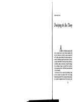
Values of λ diﬀerent from 0 move the probability mass of the N (λ, 1) distribu-
tion away from the center of the N (0, 1) distribution and into its tails. This
can be seen in Figure 4.1, which graphs the N (0, 1) density and the N(λ, 1)
density for λ = 2. The second density places much more probability than the
ﬁrst on values of z greater than 2. Thus, if the rejection region for our test
was the interval from 2 to +∞, there would be a much higher probability in
that region for λ = 2 than for λ = 0. Therefore, we would reject the null
hypothesis more often when the null hypothesis is false, with λ = 2, than
when it is true, with λ = 0.
2
Another term that often arises in the discussion of hypothesis testing is the size
of a test. Technically, this is the supremum of the rejection probability over all
DGPs that satisfy the null hypothesis. For an exact test, the size equals the
level. For an approximate test, the size is typically diﬃcult or impossible to
calculate. It is often, but by no means always, greater than the nominal level
of the test.
Copyright

c
 1999, Russell Davidson and James G. MacKinnon
4.2 Basic Ideas 127
−3 −2 −1 0 1 2 3 4 5
0.0
0.1
0.2
0.3
0.4

.

.

.
.

.
.

.
.

.
.

.
.

.
.

.
.

.
.

.
.

.
.

.
.

.
.

.
.

.
.

.
.

.
.

.
.
.

.
.
.

.
.
.

.
.
.

.
.
.

.

.
.

.
.
.

.
.
.

.
.
.

.
.
.
.

.
.
.
.

.
.
.
.

.
.
.
.

.
.
.
.
.

.
.
.
.
.

.
.
.
.
.

.
.
.
.
.
.

.
.
.
.
.
.

.
.
.
.
.
.

.
.
.
.
.
.
.

.
.
.
.
.
.
.

.
.
.
.
.
.
.
.

.
.
.
.
.
.
.
.

.
.
.
.
.
.
.
.

.
.
.

.
.
.
.
.
.

.
.
.
.
.
.
.
.
.

.
.
.
.
.
.
.
.
.

.
.
.

.
.
.
.
.
.
.

.
.
.
.
.
.
.
.
.
.

.
.
.
.
.
.
.
.
.
.

.
.
.
.
.
.
.
.
.
.

.
.
.
.
.
.
.
.
.
.

.
.
.
.
.
.
.
.

.
.
.

.
.
.
.
.
.
.
.
.
.
.

.
.
.
.
.
.
.
.
.
.
.

.
.

.
.
.
.
.
.
.
.
.

.
.
.
.
.
.
.
.
.
.

.
.
.
.
.
.
.
.
.

.

.
.
.
.
.
.
.
.
.
.

.
.
.
.
.
.
.
.
.
.

.
.
.
.
.
.

.
.
.

.
.
.
.
.
.
.
.
.

.
.
.
.
.
.
.
.

.
.
.
.
.
.
.

.

.
.
.
.
.
.
.

.
.
.
.
.
.
.

.
.
.
.
.
.

.
.
.
.
.

.
.
.
.
.

.
.
.
.

.
.
.
.

.
.
.

.
.
.

.
.

.
.

.
.
.

.
.
.

.
.
.
.

.
.
.
.

.
.
.
.
.

.
.
.
.
.

.
.
.
.
.
.

.
.
.
.
.
.
.

.
.
.
.
.
.
.

.
.
.
.
.
.

.
.

.
.
.
.
.
.
.
.

.
.
.
.
.
.
.
.
.

.
.
.
.
.
.
.
.

.

.
.
.
.
.
.
.
.
.
.

.
.
.
.
.
.
.
.
.
.

.
.
.
.
.
.

.
.
.
.

.
.
.
.
.
.
.
.
.
.

.
.
.
.
.
.
.
.
.
.
.

.
.

.
.
.
.
.
.
.
.
.

.
.
.
.
.
.
.
.
.
.
.

.
.
.
.
.
.
.
.

.
.
.

.
.
.
.
.
.
.
.
.
.

.
.
.
.
.
.
.
.
.
.

.
.
.
.

.
.
.
.
.
.

.
.
.
.
.
.
.
.
.
.

.
.
.
.
.
.
.
.
.
.

.

.
.
.
.
.
.
.
.

.
.
.
.
.
.
.
.
.

.
.
.
.
.
.
.
.
.

.

.
.
.
.
.
.
.

.
.
.
.
.
.
.
.

.
.
.
.
.
.
.
.

.
.
.
.

.
.
.

.
.
.
.
.
.
.

.
.
.
.
.
.

.
.
.
.
.
.

.
.
.
.

.
.

.
.
.
.
.

.
.
.
.
.

.
.
.
.
.

.
.
.
.

.
.
.
.

.
.
.
.

.
.
.
.

.
.
.

.
.
.

.
.
.

.
.
.

.
.
.

.
.
.

.
.
.

.
.
.

.
.
.

.
.

.
.

.
.

.
.

.

.

.
.

.
.

.
.

.
.

.
.

.
.

.
.

.
.

.
.

.

.

.
.

.
.
.
.
.

.

z
φ(z)

.
.
.
.
.
.
.
.
.

.
.
.
.
.
.
.
.
.
.
.
.
.
.
.
.
.
.
.
.
.
.
.
.
.
.
.
.
.
.

.
.
.
.
.
.
.
.
.
.
.
.
.
.
.
.
.
.
.
.
λ = 0

.

.

.
.

.
.

.
.

.
.

.
.

.
.

.
.

.
.

.
.

.
.

.
.

.
.

.
.

.
.

.
.

.
.

.
.
.

.
.
.

.

.
.

.
.
.

.
.
.

.
.
.

.
.
.

.
.
.

.
.
.

.
.
.

.

.
.
.
.

.
.
.
.

.
.
.
.

.
.
.
.
.

.
.
.
.
.

.

.
.
.
.

.
.
.
.
.
.

.
.
.
.
.
.

.
.
.
.
.
.

.
.
.
.

.
.
.

.
.
.
.
.
.
.

.
.
.
.
.
.
.
.

.
.
.
.
.
.
.
.

.
.
.
.
.
.
.
.

.
.
.
.
.
.
.
.
.

.
.
.
.
.
.
.
.
.

.

.
.
.
.
.
.
.
.

.
.
.
.
.
.
.
.
.
.

.
.
.
.
.
.
.
.
.
.

.
.
.
.
.
.
.
.
.
.

.
.
.
.
.
.
.
.
.
.

.
.
.
.
.
.
.

.
.
.

.
.
.
.
.
.
.
.
.
.
.

.
.
.
.
.
.
.
.
.
.
.

.
.

.
.
.
.
.
.
.
.
.

.
.
.
.
.
.
.
.
.
.
.

.
.
.
.
.
.
.
.

.
.

.
.
.
.
.
.
.
.
.
.

.
.
.
.
.
.
.
.
.
.

.
.
.
.
.

.
.
.
.
.

.
.
.
.
.
.
.
.
.

.
.
.
.
.
.
.
.
.

.
.
.
.

.
.
.
.

.
.
.
.
.
.
.
.

.
.
.
.
.
.
.

.
.
.
.
.
.
.

.
.
.
.
.
.

.
.
.
.
.

.
.
.
.
.

.
.
.
.

.
.
.
.

.

.
.

.
.
.

.
.

.
.

.
.
.

.
.
.

.
.
.
.

.
.
.
.

.
.
.
.
.

.
.
.
.
.

.
.
.
.
.
.

.
.
.
.
.
.
.

.
.

.
.
.
.
.

.
.
.
.
.
.
.
.

.
.
.
.
.
.
.
.

.
.
.
.
.
.

.
.
.

.
.
.
.
.
.
.
.
.

.
.
.
.
.
.
.
.
.
.

.
.
.
.
.

.
.
.
.
.

.
.
.
.
.
.
.
.
.
.

.
.
.
.
.
.
.
.
.
.

.
.

.
.
.
.
.
.
.
.
.

.
.
.
.
.
.
.
.
.
.
.

.
.
.
.
.
.
.
.

.
.
.

.
.
.
.
.
.
.
.
.
.
.

.
.
.
.
.
.
.
.
.
.

.
.
.

.
.
.
.
.
.
.

.
.
.
.
.
.
.
.
.
.

.
.
.
.
.
.
.
.
.
.

.
.
.
.
.
.
.
.
.
.

.
.
.
.
.
.
.
.
.

.
.
.
.
.
.
.
.
.

.
.
.
.
.
.
.
.
.

.
.
.
.
.
.
.
.

.
.
.
.
.
.
.
.

.

.
.
.
.
.
.
.

.
.
.
.
.
.
.

.
.
.
.
.
.
.

.
.
.
.
.
.

.
.
.
.
.
.

.
.
.
.
.
.

.
.
.
.
.

.
.
.
.
.

.
.
.

.
.

.
.
.
.

.
.
.
.

.
.
.
.

.
.
.
.

.
.
.

.
.
.

.
.
.

.
.
.

.
.
.

.
.
.

.
.
.

.
.
.

.
.
.

.

.

.
.

.
.

.
.

.
.

.
.

.
.

.
.

.
.

.
.

.

.

.
.

.
.

.
.

.
.

.
.

.
.
.
.
.

.

.
.
.
.
.
.
.
.
.
.
.
.
.
.
.
.
.
.
.
.
.
.
.
.
.
.
.
.
.

.
.
.
.
.
.
.
.
.
.
.
.
.
.
.
.
.
.
.
.
.
.
.
.
.
.
.
.
.
.

λ = 2
.
.
.
.
.
.
.
.
.
.
.
.
.
.
.
.
.
.
.
.
.
.
.
.
.
.
.
.
.

.
.
.
.
.
.
.
.
.
.
.
.
.
.
.
.
.
.
.
.
.
.
.
.
.
.
.
.
.
.

.
.
.
Figure 4.1 The normal distribution centered and uncentered
Mistakenly failing to reject a false null hypothesis is called making a Type II
error. The probability of making such a mistake is equal to 1 minus the
power of the test. It is not hard to see that, quite generally, the probability of
rejecting the null with a two-tailed test based on z increases with the absolute
value of λ. Consequently, the power of such a test will increase as β
1
− β
0
increases, as σ decreases, and as the sample size increases. We will discuss
what determines the power of a test in more detail in Section 4.7.
In order to construct the rejection region for a test at level α, the ﬁrst step
is to calculate the critical value associated with the level α. For a two-tailed
test based on any test statistic that is distributed as N(0, 1), including the
statistic z deﬁned in (4.04), the critical value c
α
is deﬁned implicitly by
Φ(c
α
) = 1 −α/2. (4.05)
Recall that Φ denotes the CDF of the standard normal distribution. In terms
of the inverse function Φ
−1
, c
α
can b e deﬁned explicitly by the formula
c

α
= Φ
−1
(1 − α/2). (4.06)
According to (4.05), the probability that z > c
α
is 1 − (1 − α/2) = α/2, and
the probability that z < −c
α
is also α/2, by symmetry. Thus the probability
that |z| > c
α
is α, and so an appropriate rejection region for a test at level α
is the set deﬁned by |z| > c
α
. Clearly, c
α
increases as α approaches 0. As
an example, when α = .05, we see from (4.06) that the critical value for a
two-tailed test is Φ
−1
(.975) = 1.96. We would reject the null at the .05 level
whenever the observed absolute value of the test statistic exceeds 1.96.
P Values
As we have deﬁned it, the result of a test is yes or no: Reject or do not
reject. A more sophisticated approach to deciding whether or not to reject
Copyright
c
 1999, Russell Davidson and James G. MacKinnon
128 Hypothesis Testing in Linear Regression Models

the null hypothesis is to calculate the P value, or marginal signiﬁcance level,
associated with the observed test statistic ˆz. The P value for ˆz is deﬁned as the
greatest level for which a test based on ˆz fails to reject the null. Equivalently,
at least if the statistic z has a continuous distribution, it is the smallest level
for which the test rejects. Thus, the test rejects for all levels greater than the
P value, and it fails to reject for all levels smaller than the P value. Therefore,
if the P value associated with ˆz is denoted p(ˆz), we must be prepared to accept
a probability p(ˆz) of Type I error if we choose to reject the null.
For a two-tailed test, in the special case we have been discussing,
p(ˆz) = 2

1 − Φ(|ˆz|)

. (4.07)
To see this, note that the test based on ˆz rejects at level α if and only if
|ˆz| > c
α
. This inequality is equivalent to Φ(|ˆz|) > Φ(c
α
), because Φ(·) is
a strictly increasing function. Further, Φ(c
α
) = 1 − α/2, by (4.05). The
smallest value of α for which the inequality holds is thus obtained by solving
the equation
Φ(|ˆz|) = 1 − α/2,
and the solution is easily seen to be the right-hand side of (4.07).
One advantage of using P values is that they preserve all the information
conveyed by a test statistic, while presenting it in a way that is directly
interpretable. For example, the test statistics 2.02 and 5.77 would both lead

us to reject the null at the .05 level using a two-tailed test. The second of
these obviously provides more evidence against the null than does the ﬁrst,
but it is only after they are converted to P values that the magnitude of the
diﬀerence becomes apparent. The P value for the ﬁrst test statistic is .0434,
while the P value for the second is 7.93 × 10
−9
, an extremely small number.
Computing a P value transforms z from a random variable with the N(0, 1)
distribution into a new random variable p(z) with the uniform U(0, 1) dis-
tribution. In Exercise 4.1, readers are invited to prove this fact. It is quite
possible to think of p(z) as a test statistic, of which the observed realization
is p(ˆz). A test at level α rejects whenever p(ˆz) < α. Note that the sign of
this inequality is the opposite of that in the condition |ˆz| > c
α
. Generally,
one rejects for large values of test statistics, but for small P values.
Figure 4.2 illustrates how the test statistic ˆz is related to its P value p(ˆz).
Suppose that the value of the test statistic is 1.51. Then
Pr(z > 1.51) = Pr(z < −1.51) = .0655. (4.08)
This implies, by equation (4.07), that the P value for a two-tailed test based
on ˆz is .1310. The top panel of the ﬁgure illustrates (4.08) in terms of the
PDF of the standard normal distribution, and the bottom panel illustrates it
in terms of the CDF. To avoid clutter, no critical values are shown on the
Copyright
c
 1999, Russell Davidson and James G. MacKinnon
4.2 Basic Ideas 129
−3 −2 −1 0 1 2 3
0.0
0.1

0.2
0.3
0.4

.

.

.

.
.

.

.
.

.
.

.

.
.
.

.
.
.

.
.
.

.
.
.

.
.
.

.
.
.

.
.
.

.
.
.

.
.
.

.
.
.

.
.
.

.
.
.

.
.
.

.
.
.

.
.

.
.

.
.
.
.

.
.
.
.

.
.
.
.

.
.
.
.

.
.
.
.

.
.

.
.

.
.
.
.

.
.
.
.

.
.
.
.

.
.
.
.
.

.
.
.
.
.

.
.
.
.
.

.
.
.
.
.

.
.
.
.
.
.

.
.
.
.
.
.

.
.
.
.

.
.

.
.
.
.
.
.

.
.
.
.
.
.
.

.
.
.
.
.
.
.

.
.
.
.

.
.
.

.
.
.
.
.
.
.

.
.
.
.
.
.
.
.

.
.
.
.
.
.
.
.

.
.
.
.
.
.
.
.

.
.
.
.
.
.
.
.

.
.
.
.
.
.
.
.

.
.
.

.
.
.
.
.
.

.
.
.
.
.
.
.
.
.

.
.
.
.
.
.
.
.
.

.
.
.

.
.
.
.
.
.

.
.
.
.
.
.
.
.
.

.
.
.
.
.
.
.
.

.
.
.
.

.
.
.
.

.
.
.
.
.
.
.
.

.
.
.
.
.
.
.
.

.
.
.
.
.
.
.

.
.
.
.
.
.
.

.
.
.
.
.
.

.
.
.
.
.
.

.
.
.
.
.
.

.
.
.
.
.

.
.
.
.
.

.
.
.
.

.
.
.
.

.
.
.
.

.
.
.

.
.
.

.
.
.

.
.
.

.
.
.
.

.
.
.
.

.
.
.
.

.
.

.
.
.

.
.
.
.
.

.
.
.
.
.
.

.
.
.
.
.
.

.
.
.
.
.
.

.
.
.
.
.
.
.

.
.
.
.
.
.
.

.
.
.
.
.
.
.
.

.
.
.
.

.
.
.
.

.
.
.
.
.
.
.
.

.
.
.
.
.
.
.
.

.
.
.
.
.
.
.

.
.

.
.
.
.
.
.
.
.
.

.
.
.
.
.
.
.
.
.

.
.
.
.
.
.
.

.
.

.
.
.
.
.
.
.
.
.

.
.
.
.
.
.
.
.

.
.
.
.
.
.
.
.

.
.
.
.
.
.
.
.

.
.
.
.
.
.
.
.

.
.
.
.
.
.
.
.

.
.

.
.
.
.
.

.
.
.
.
.
.
.

.
.
.
.
.
.
.

.
.
.
.
.
.
.

.
.
.
.
.
.

.
.
.
.
.
.

.
.
.
.
.
.

.
.
.
.
.
.

.
.

.
.
.

.
.
.
.
.

.
.
.
.
.

.
.
.
.
.

.
.
.
.

.
.
.

.

.
.
.
.

.
.
.
.

.
.
.
.

.
.
.
.

.
.
.
.

.
.
.

.

.
.
.
.

.
.
.
.

.
.
.

.
.
.

.
.
.

.
.
.

.
.

.

.
.
.

.
.
.

.
.
.

.
.
.

.
.
.

.
.
.

.
.
.

.
.
.

.
.
.

.
.
.

.
.
.

.
.
.

.
.

.
.

.
z
φ(z)
.
.
.
.
.
.
.
.
.
.
.
.
.
.
.
.
.
.
.
.
.

.
.
.
.
.
.
.
.
.
.
.
.
.
.
.
.
.
.
.
.
.
.
.
.
.
.
.
.
.
.

.
.
.

.
.
.
.
.
.
.
.
.
.
.
.
.
.
.
.
.
.
.
.
.
.
.
.
.
.

.
.
.
.
.
.
.
.
.
.
.
.
.
.
.
.
.
.
.
.
.
.
.
.
.
.
.
.
.
.

.
.
.
P = .0655
.
.
.
.
.
.
.
.
.
.
.
.
.
.
.
.
.
.
.
.
.
.
.
.
.
.

.
.
.
.
.
.
.
.
.
.
.
.
.
.
.
.
.
.
.
.
.
.
.
.
.
.
.
.
.
.

.
.
.
.
.
.
.
.
.
.
.
.
.
.
.
.
.
.

.
.
.
.
.
.
.
.
.
.
.

.
.
.
.
.
.
.
.
.
.
.
.
.
.
.
.
.
.
.
.
.
.
.
.
.
.
.
.
.
.

.
.
.
.
.
.
.
.
.
.
.
.
.
.
.
.
.
.
P = .0655

.

.
.
.

.
.
.

.
.
.

.
.
.

.
.
.

.
.
.

.
.
.

.
.
.

.
.
.

.
.
.

.
.
.

.
.
.

.

.
.

.
.
.

.
.
.

.
.
.

.
.
.

.
.
.

.
.
.

.
.
.

.
.
.

.
.
.
.

.
.
.
.

.
.
.
.

.
.
.
.

.
.
.
.

.
.
.
.

.
.
.
.

.
.
.
.

.
.
.
.

.
.
.
.

.
.
.
.

.
.
.
.
.

.
.
.
.
.

.
.
.
.
.

.
.
.
.
.

.
.
.
.
.

.
.
.
.
.

.
.
.
.
.
.

.
.
.
.
.
.

.
.
.
.
.
.

.
.
.

.
.
.

.
.
.
.
.
.

.
.
.
.
.
.

.
.
.
.
.
.

.
.
.
.
.

.
.

.
.
.
.
.
.
.

.
.
.
.
.
.
.

.
.
.
.
.
.
.

.
.
.

.
.
.
.

.
.
.
.
.
.
.

.
.
.
.
.
.
.

.
.
.
.
.
.
.

.

.
.
.
.
.
.

.
.
.
.
.
.
.

.
.
.
.
.
.
.

.
.
.
.
.
.
.

.
.
.
.
.
.
.

.
.
.
.
.
.
.

.
.
.
.
.
.
.

.
.
.
.
.

.
.

.
.
.
.
.
.
.

.
.
.
.
.
.
.

.
.
.
.
.
.
.

.
.
.

.
.
.
.

.
.
.
.
.
.
.

.
.
.
.
.
.
.

.
.
.
.
.
.

.
.

.
.
.
.

.
.
.
.
.
.

.
.
.
.
.
.

.
.
.
.
.
.

.
.
.
.

.
.

.
.
.
.
.
.

.
.
.
.
.

.
.
.
.
.

.
.
.
.
.

.
.

.
.
.

.
.
.
.
.

.
.
.
.
.

.
.
.
.

.
.
.
.

.
.
.
.

.
.
.
.

.
.
.
.

.
.
.
.

.
.
.
.

.
.
.
.

.
.
.
.

.
.
.
.

.
.
.
.

.
.
.

.
.
.

.
.
.

.
.
.

.
.
.

.
.
.

.
.
.

.
.
.

.
.
.

.
.
.

.
.
.

.
.
.

.

.
.

.
.
.

.
.
.

.
.
.

.
.
.

.
.
.

.
.
.

.

.
.

.

.
.
.
.
.

.
.
.
.
.
.
.
.
.
.
.
.
.
.
.
.
.
.
.
.
.
.
.
.
.
.
.
.
.
.

.
.
.
.
.
.

.
.
.
.
.

1.51
−1.51
0.9345
0.0655
Φ(z)
z
Figure 4.2 P values for a two-tailed test
ﬁgure, but it is clear that a test based on ˆz will not reject at any level smaller
than .131. From the ﬁgure, it is also easy to see that the P value for a one-
tailed test of the hypothesis that β ≤ β
0
is .0655. This is just Pr(z > 1.51).
Similarly, the P value for a one-tailed test of the hypothesis that β ≥ β
0
is
Pr(z < 1.51) = .9345.
In this section, we have introduced the basic ideas of hypothesis testing. How-

ever, we had to make two very restrictive assumptions. The ﬁrst is that the
error terms are normally distributed, and the second, which is grossly unreal-
istic, is that the variance of the error terms is known. In addition, we limited
our attention to a single restriction on a single parameter. In Section 4.4, we
will discuss the more general case of linear restrictions on the parameters of
a linear regression model with unknown error variance. Before we can do so,
however, we need to review the properties of the normal distribution and of
several distributions that are closely related to it.
Copyright
c
 1999, Russell Davidson and James G. MacKinnon
130 Hypothesis Testing in Linear Regression Models
4.3 Some Common Distributions
Most test statistics in econometrics follow one of four well-known distribu-
tions, at least approximately. These are the standard normal distribution,
the chi-squared (or χ
2
) distribution, the Student’s t distribution, and the
F distribution. The most basic of these is the normal distribution, since the
other three distributions can be derived from it. In this section, we discuss the
standard, or central, versions of these distributions. Later, in Section 4.7, we
will have occasion to introduce noncentral versions of all these distributions.
The Normal Distribution
The normal distribution, which is sometimes called the Gaussian distribu-
tion in honor of the celebrated German mathematician and astronomer Carl
Friedrich Gauss (1777–1855), even though he did not invent it, is certainly
the most famous distribution in statistics. As we saw in Section 1.2, there
is a whole family of normal distributions, all based on the standard normal
distribution, so called because it has mean 0 and variance 1. The PDF of the
standard normal distribution, which is usually denoted by φ(·), was deﬁned

in (1.06). No elementary closed-form expression exists for its CDF, which is
usually denoted by Φ(·). Although there is no closed form, it is perfectly easy
to evaluate Φ numerically, and virtually every program for doing econometrics
and statistics can do this. Thus it is straightforward to compute the P value
for any test statistic that is distributed as standard normal. The graphs of
the functions φ and Φ were ﬁrst shown in Figure 1.1 and have just reappeared
in Figure 4.2. In both tails, the PDF rapidly approaches 0. Thus, although
a standard normal r.v. can, in principle, take on any value on the real line,
values greater than about 4 in absolute value occur extremely rarely.
In Exercise 1.7, readers were asked to show that the full normal family can be
generated by varying exactly two parameters, the mean and the variance. A
random variable X that is normally distributed with mean µ and variance σ
2
can b e generated by the formula
X = µ + σZ, (4.09)
where Z is standard normal. The distribution of X, that is, the normal
distribution with mean µ and variance σ
2
, is denoted N(µ, σ
2
). Thus the
standard normal distribution is the N(0, 1) distribution. As readers were
asked to show in Exercise 1.8, the PDF of the N (µ, σ
2
) distribution, evaluated
at x, is
1
−
σ
φ


x − µ
σ

=
1
σ
√
2π
exp

−
(x − µ)
2
2σ
2

,
(4
.
10)
In expression (4.10), as in Section 1.2, we have distinguished between the
random variable X and a value x that it can take on. However, for the
following discussion, this distinction is more confusing than illuminating. For
Copyright
c
 1999, Russell Davidson and James G. MacKinnon
4.3 Some Common Distributions 131
the rest of this section, we therefore use lower-case letters to denote both
random variables and the arguments of their PDFs or CDFs, depending on

context. No confusion should result. Adopting this convention, then, we
see that, if x is distributed as N(µ, σ
2
), we can invert (4.09) and obtain
z = (x −µ)/σ, where z is standard normal. Note also that z is the argument
of φ in the expression (4.10) of the PDF of x. In general, the PDF of a
normal variable x with mean µ and variance σ
2
is 1/σ times φ evaluated at
the corresp onding standard normal variable, which is z = (x − µ)/σ.
Although the normal distribution is fully characterized by its ﬁrst two mo-
ments, the higher moments are also important. Because the distribution is
symmetric around its mean, the third central moment, which measures the
skewness of the distribution, is always zero.
3
This is true for all of the odd
central moments. The fourth moment of a symmetric distribution provides a
way to measure its kurtosis, which essentially means how thick the tails are.
In the case of the N(µ, σ
2
) distribution, the fourth central moment is 3σ
4
; see
Exercise 4.2.
Linear Combinations of Normal Variables
An important property of the normal distribution, used in our discussion in
the preceding section, is that any linear combination of independent normally
distributed random variables is itself normally distributed. To see this, it
is enough to show it for independent standard normal variables, because,
by (4.09), all normal variables can be generated as linear combinations of

standard normal ones plus constants. We will tackle the proof in several
steps, each of which is important in its own right.
To begin with, let z
1
and z
2
be standard normal and mutually independent,
and consider w ≡ b
1
z
1
+ b
2
z
2
. For the moment, we suppose that b
2
1
+ b
2
2
= 1,
although we will remove this restriction shortly. If we reason conditionally
on z
1
, then we ﬁnd that
E(w |z
1
) = b
1

z
1
+ b
2
E(z
2
|z
1
) = b
1
z
1
+ b
2
E(z
2
) = b
1
z
1
.
The ﬁrst equality follows because b
1
z
1
is a deterministic function of the condi-
tioning variable z
1
, and so can be taken outside the conditional expectation.
The second, in which the conditional expectation of z

2
is replaced by its un-
conditional expectation, follows because of the independence of z
1
and z
2
(see
Exercise 1.9). Finally, E(z
2
) = 0 because z
2
is N(0, 1).
The conditional variance of w is given by
E


w −E(w |z
1
)

2


z
1

= E

(b
2

z
2
)
2
|z
1

= E

(b
2
z
2
)
2

= b
2
2
,
3
A distribution is said to be skewed to the right if the third central moment is
positive, and to the left if the third central moment is negative.
Copyright
c
 1999, Russell Davidson and James G. MacKinnon
132 Hypothesis Testing in Linear Regression Models
where the last equality again follows because z
2
∼ N(0, 1). Conditionally

on z
1
, w is the sum of the constant b
1
z
1
and b
2
times a standard normal
variable z
2
, and so the conditional distribution of w is normal. Given the
conditional mean and variance we have just computed, we see that the con-
ditional distribution must be N( b
1
z
1
, b
2
2
). The PDF of this distribution is the
density of w conditional on z
1
, and, by (4.10), it is
f(w |z
1
) =
1
b
2

φ

w −b
1
z
1
b
2

. (4.11)
In accord with what we noted above, the argument of φ here is equal to z
2
,
which is the standard normal variable corresponding to w conditional on z
1
.
The next step is to ﬁnd the joint density of w and z
1
. By (1.15), the density
of w conditional on z
1
is the ratio of the joint density of w and z
1
to the
marginal density of z
1
. This marginal density is just φ(z
1
), since z
1

∼ N(0, 1),
and so we see that the joint density is
f(w, z
1
) = f (z
1
) f (w |z
1
) = φ(z
1
)
1
b
2
φ

w −b
1
z
1
b
2

. (4.12)
If we use (1.06) to get an explicit expression for this joint density, then we
obtain
1
2πb
2
exp


−
1
2b
2
2

b
2
2
z
2
1
+ w
2
− 2b
1
z
1
w + b
2
1
z
2
1


=
1
2πb

2
exp

−
1
2b
2
2

z
2
1
− 2b
1
z
1
w + w
2


,
(4.13)
since we assumed that b
2
1
+ b
2
2
= 1. The right-hand side of (4.13) is symmetric
with respect to z

1
and w. Thus the joint density can also be expressed as
in (4.12), but with z
1
and w interchanged, as follows:
f(w, z
1
) =
1
b
2
φ(w)φ

z
1
− b
1
w
b
2

. (4.14)
We are now ready to compute the unconditional, or marginal, density of w.
To do so, we integrate the joint density (4.14) with respect to z
1
; see (1.12).
Note that z
1
occurs only in the last factor on the right-hand side of (4.14).
Further, the expression (1/b

2
)φ

(z
1
− b
1
w)/b
2

, like expression (4.11), is a
probability density, and so it integrates to 1. Thus we conclude that the
marginal density of w is f (w) = φ(w), and so it follows that w is standard
normal, unconditionally, as we wished to show.
It is now simple to extend this argument to the case for which b
2
1
+ b
2
2
= 1.
We deﬁne r
2
= b
2
1
+ b
2
2
, and consider w/r. The argument above shows that

w/r is standard normal, and so w ∼ N(0, r
2
). It is equally simple to extend
the result to a linear combination of any number of mutually independent
standard normal variables. If we now let w be deﬁned as b
1
z
1
+ b
2
z
2
+ b
3
z
3
,
Copyright
c
 1999, Russell Davidson and James G. MacKinnon
4.3 Some Common Distributions 133
where z
1
, z
2
, and z
3
are mutually independent standard normal variables, then
b
1

z
1
+b
2
z
2
is normal by the result for two variables, and it is independent of z
3
.
Thus, by applying the result for two variables again, this time to b
1
z
1
+ b
2
z
2
and z
3
, we see that w is normal. This reasoning can obviously be extended
by induction to a linear combination of any number of independent standard
normal variables. Finally, if we consider a linear combination of independent
normal variables with nonzero means, the mean of the resulting variable is
just the same linear combination of the means of the individual variables.
The Multivariate Normal Distribution
The results of the previous subsection can be extended to linear combina-
tions of normal random variables that are not necessarily independent. In
order to do so, we introduce the multivariate normal distribution. As the
name suggests, this is a family of distributions for random vectors, with the
scalar normal distributions being special cases of it. The pair of random

variables z
1
and w considered above follow the bivariate normal distribution,
another special case of the multivariate normal distribution. As we will see
in a moment, all these distributions, like the scalar normal distribution, are
completely characterized by their ﬁrst two moments.
In order to construct the multivariate normal distribution, we begin with a
set of m mutually independent standard normal variables, z
i
, i = 1, . . . , m,
which we can assemble into a random m vector z. Then any m vector x
of linearly independent linear combinations of the components of z follows
a multivariate normal distribution. Such a vector x can always be written
as Az, for some nonsingular m × m matrix A. As we will see in a moment,
the matrix A can always be chosen to be lower-triangular.
We denote the components of x as x
i
, i = 1, . . . , m. From what we have seen
above, it is clear that each x
i
is normally distributed, with (unconditional)
mean zero. Therefore, from results proved in Section 3.4, it follows that the
covariance matrix of x is
Var(x ) = E(xx

) = AE(zz

)A

= AIA


= AA

.
Here we have used the fact that the covariance matrix of z is the identity
matrix I. This is true because the variance of each component of z is 1,
and, since the z
i
are mutually independent, all the covariances are 0; see
Exercise 1.11.
Let us denote the covariance matrix of x by Ω. Recall that, according to
a result mentioned in Section 3.4 in connection with Crout’s algorithm, for
any positive deﬁnite matrix Ω, we can always ﬁnd a lower-triangular A such
that AA

= Ω. Thus the matrix A may always be chosen to be lower-
triangular. The distribution of x is multivariate normal with mean vector 0
and covariance matrix Ω. We write this as x ∼ N(0, Ω). If we add an
m vector µ of constants to x, the resulting vector must follow the N(µ, Ω)
distribution.
Copyright
c
 1999, Russell Davidson and James G. MacKinnon
134 Hypothesis Testing in Linear Regression Models
x
2
x
1
.
.

.

.

.

.

.

.

.

.

.

.

.

.

.

.

.

.

.

.

.

.

.

.

.

.

.

.
.
.
.

.

.

.

.

.

.

.

.

.

.

.

.

.

.

.

.

.

.

.

.

.

.

.

.

.

.

.

.

.

.

.

.
.
.
.

.

.

.

.

.

.

.

.

.

.

.

.

.

.

.

.

.

.

.

.

.

.

.

.

.

.

.

.

.

.

.
.
.
.

.

.

.

.

.

.

.

.

.

.

.

.

.

.

.

.

.

.

.

.

.

.

.

.

.

.

.

.

.

.

.

.

.

.

.

.

.

.

.

.

.

.

.

.

.

.

.

.

.

.

.

.

.

.

.

.
.
.
.
.
.
.

.
.
.
.

.
.
.
.

.
.
.
.

.
.

.
.

.
.
.
.

.
.
.
.

.
.
.
.

.
.
.
.

.
.
.
.

.
.

.
.

.

.
.
.
.

.
.
.
.

.
.
.
.

.
.
.
.

.
.

.
.

.
.
.
.

.
.
.
.

.
.
.
.

.
.
.
.

.
.
.
.

.
.

.
.

.
.
.

.
.
.
.

.
.
.
.

.
.
.
.

.
.
.
.

.
.
.

.

.
.
.
.

.
.
.
.

.
.
.
.

.
.
.
.

.
.
.
.

.
.
.

.

.
.
.
.
.
.
.

.
.
.
.

.
.
.
.

.
.
.
.

.
.
.
.

.
.
.
.

.
.
.
.

.
.
.
.

.
.
.
.

.
.
.
.

.
.
.
.

.
.
.
.

.
.
.
.

.
.

.
.
.
.

.
.
.
.

.
.
.
.

.
.
.
.

.
.
.
.

.
.
.
.

.
.
.
.

.
.
.
.

.
.
.
.

.
.
.
.

.
.
.
.

.
.
.
.

.
.
.
.

.
.
.
.

.
.
.
.

.
.
.
.

.
.
.
.

.
.
.
.

.
.
.
.

.
.
.
.

.
.
.
.
.
.
.

.
.
.
.

.
.
.
.

.
.
.
.

.
.
.
.

.

.
.
.

.
.
.
.

.
.
.
.

.
.
.
.

.
.
.
.

.
.
.
.

.

.
.
.

.
.
.
.

.
.
.
.

.
.
.
.

.
.
.
.

.
.
.

.
.

.
.
.
.

.
.
.
.

.
.
.
.

.
.
.
.

.
.
.
.

.

.
.
.

.
.
.
.

.
.
.
.

.
.
.
.

.
.
.
.

.
.
.
.

.

.
.
.

.
.
.
.

.
.
.

.
.
.

.
.
.
.

.
.
.
.

.
.
.
.

.
.
.
.

.
.
.
.

.
.
.
.

.
.
.
.

.
.
.
.

.
.
.
.
.
.
.
.
.
.

.
.
.
.

.
.
.
.

.
.
.
.

.
.
.
.

.
.
.
.

.
.
.
.

.
.
.
.

.
.
.
.

.
.
.
.

.
.
.
.

.
.
.
.

.
.
.
.

.
.
.
.

.
.

.

.
.
.
.

.

.
.
.

.
.
.
.

.
.
.
.

.
.
.
.

.
.
.
.

.
.
.
.

.

.
.
.

.
.
.
.

.

.

.
.
.
.

.
.
.
.

.
.

.
.

.
.
.
.

.
.
.
.

.
.
.
.

.
.
.
.

.
.
.
.

.
.

.
.

.
.
.
.

.
.
.
.

.
.
.
.

.
.
.
.
.
σ
1
= 1, σ
2
= 1, ρ = 0.5
.
.

.

.

.

.

.

.

.

.

.

.

.

.

.

.

.

.

.

.

.

.

.

.

.

.
.
.
.

.

.

.

.

.

.

.

.

.

.

.

.

.

.

.

.

.

.

.

.

.

.

.

.

.

.

.

.

.
.
.
.
.
.
.

.
.
.
.

.
.
.
.

.
.
.
.

.
.
.
.

.
.
.
.

.
.
.
.

.
.
.
.

.
.
.
.

.
.
.
.

.
.
.
.

.
.
.
.

.
.
.
.

.
.
.

.

.
.

.
.
.

.
.
.

.
.
.
.

.

.
.
.
.

.
.
.
.

.

.
.
.

.
.
.
.

.
.
.
.

.
.
.
.

.
.
.
.

.
.
.
.

.

.
.
.

.
.
.

.
.
.

.
.
.

.
.
.

.
.
.
.

.
.
.

.

.
.
.
.

.
.
.
.

.
.
.
.

.
.
.
.

.
.
.
.

.
.
.

.

.
.
.
.

.
.
.
.
.
.
.

.
.
.
.

.
.
.
.

.
.
.
.

.
.
.
.

.
.
.
.

.
.
.
.

.
.
.
.

.
.
.
.

.
.
.
.

.
.
.
.

.
.
.
.

.
.
.
.

.
.
.
.

.
.
.
.

.
.
.

.

.
.

.
.
.

.
.
.
.

.
.
.
.

.
.
.
.

.
.
.
.

.
.

.
.

.
.
.
.

.
.
.
.

.
.
.
.

.
.
.
.

.
.
.
.

.
.

.
.

.
.
.
.

.
.
.
.

.
.
.
.

.
.
.
.

.
.
.

.
.
.

.
.
.

.
.
.

.
.
.
.

.
.
.
.

.
.
.
.

.
.
.
.

.

.
.
.

.
.
.
.

.
.
.
.

.
.
.
.

.
.
.
.

.
.
.
.

.

.
.
.

.
.
.
.
.
.
.

.
.
.
.

.
.
.
.

.
.
.
.

.
.
.

.

.
.
.
.

.
.
.
.

.
.
.
.

.
.
.
.

.
.
.
.

.
.
.

.
.
.

.
.
.

.
.
.

.
.
.

.
.
.
.

.
.

.
.

.
.

.
.
.
.

.
.
.
.

.
.
.
.

.
.
.
.

.
.
.
.

.
.

.
.

.
.
.
.

.
.
.
.

.
.
.
.

.
.
.
.

.
.
.

.
.
.

.
.
.

.
.
.
.

.
.
.
.

.
.
.
.

.
.
.

.
.
.
.

.

.
.
.

.
.
.
.

.
.
.
.

.
.
.
.

.
.
.
.

.
.
.
.

.

.
.
.

.
.
.
.

.
.
.
.

.
.
.
.

.
.
.
.
.
.
.
.
.
.

.
.
.
.

.
.
.
.

.
.
.
.

.
.
.
.

.
.
.
.

.
.
.
.

.
.
.

.
.
.

.
.
.

.
.
.

.
.
.
.

.
.
.
.

.
.
.
.

.
.
.
.

.
.
.
.

.
.
.
.

.
.
.
.

.
.
.
.

.
.
.
.

.
.
.
.

.
.
.
.

.
.
.

.
.
.

.
.
.

.
.
.

.
.
.
.

.
.
.
.

.
.
.
.

.
.
.
.

.
.
.
.

.
.
.

.

.
.
.
.

.
.
.
.

.
.
.
.

.
.
.
.

.
.
.
.

.
.
.

.
.
.
.

.
.
.
.

.
.
.
.

.
.
.
.

.
.
.
.

.
.
.
.

.
.
.
.

.
.
.
.

.
.
.
.

.
.
.
.

.
.
.

.
.
.

.
.

.

.
.
.

.
.
.
.

.
.
.
.

.
.
.
.

.
.
.
.

.
.
.

.
.
.
.

.
.
.
.

.
.
.
.

.
.
.
.

.
.
.
.

.
.
.
.

.
.
.
.

.
.
.
.

.
.
.
.

.
.
.

.
.
.

.
.
.

.
.
.

.
.
.

.
.
.
.

.
.
.
.

.
.
.
.

.
.
.
.

.

.
.
.

.
.
.
.

.
.
.
.

.
.
.
.

.
.
.
.

.
.
.
.

.

.
.
.

.
.
.
.

.
.
.
.

.
.
.
.

.
.
.
.
.
.
.
.
.
.

.
.
.
.

.
.
.
.

.
.
.
.

.
.
.
.

.
.
.
.

.
.
.
.

.
.
.
.

.
.
.
.

.
.
.
.

.
.
.
.

.
.
.
.

.
.
.

.

.
.

.
.
.

.
.
.
.

.
.
.
.

.
.
.
.

.
.
.
.

.
.
.
.

.
.
.
.

.
.
.
.

.
.
.
.

.
.
.
.

.
.
.
.

.
.
.
.

.
.
.
.

.
.
.
.

.
.
.
.

.
.
.
.

.
.
.

.
.
.

.
.
.

.
.
.
.

.
.
.
.

.
.
.
.

.
.
.
.

.
.

.
.

.
.
.
.

.
.
.
.

.
.
.
.

.
.
.
.

.
.
.
.

.
.
.
.

.
.
.
.

.
.
.
.

.
.
.
.

.
.
.
.

.
.
.
.

.
.
.
.

.
.
σ
1
= 1.5, σ
2
= 1, ρ = −0.9
Figure 4.3 Contours of two bivariate normal densities
It is clear from this argument that any linear combination of random variables
that are jointly multivariate normal is itself normally distributed. Thus, if
x ∼ N(µ, Ω), any scalar a

x, where a is an m vector of ﬁxed coeﬃcients, is
normally distributed with mean a

µ and variance a

Ωa.
We saw a moment ago that z ∼ N(0, I) whenever the components of the
vector z are independent. Another crucial property of the multivariate nor-
mal distribution is that the converse of this result is also true: If x is any
multivariate normal vector with zero covariances, the components of x are
mutually independent. This is a very special property of the multivariate
normal distribution, and readers are asked to prove it, for the bivariate case,

in Exercise 4.5. In general, a zero covariance between two random variables
does not imply that they are independent.
It is important to note that the results of the last two paragraphs do not hold
unless the vector x is multivariate normal, that is, constructed as a set of linear
combinations of independent normal variables. In most cases, when we have
to deal with linear combinations of two or more normal random variables, it is
reasonable to assume that they are jointly distributed as multivariate normal.
However, as Exercise 1.12 illustrates, it is possible for two or more random
variables not to be multivariate normal even though each one individually
follows a normal distribution.
Figure 4.3 illustrates the bivariate normal distribution, of which the PDF is
given in Exercise 4.5 in terms of the variances σ
2
1
and σ
2
2
of the two variables,
and their correlation ρ. Contours of the density are plotted, on the right for
σ
1
= σ
2
= 1.0 and ρ = 0.5, on the left for σ
1
= 1.5, σ
2
= 1.0, and ρ = −0.9.
The contours of the bivariate normal density can be seen to be elliptical. The
ellipses slope upward when ρ > 0 and downward when ρ < 0. They do so

Copyright
c
 1999, Russell Davidson and James G. MacKinnon
4.3 Some Common Distributions 135
more steeply the larger is the ratio σ
2
/σ
1
. The closer |ρ| is to 1, for given
values of σ
1
and σ
2
, the more elongated are the elliptical contours.
The Chi-Squared Distribution
Suppose, as in our discussion of the multivariate normal distribution, that
the random vector z is such that its components z
1
, . . . , z
m
are mutually
independent standard normal random variables. An easy way to express this
is to write z ∼ N(0, I). Then the random variable
y ≡ z
2
= z

z =
m


i=1
z
2
i
(4.15)
is said to follow the chi-squared distribution with m degrees of freedom. A
compact way of writing this is: y ∼ χ
2
(m). From (4.15), it is clear that
m must be a positive integer. In the case of a test statistic, it will turn out
to b e equal to the number of restrictions being tested.
The mean and variance of the χ
2
(m) distribution can easily be obtained from
the deﬁnition (4.15). The mean is
E(y) =
m

i=1
E(z
2
i
) =
m

i=1
1 = m. (4.16)
Since the z
i
are independent, the variance of the sum of the z

2
i
is just the sum
of the (identical) variances:
Var(y) =
m

i=1
Var(z
2
i
) = mE

(z
2
i
− 1)
2

= mE(z
4
i
− 2z
2
i
+ 1) = m(3 − 2 + 1) = 2m.
(4.17)
The third equality here uses the fact that E(z
4
i

) = 3; see Exercise 4.2.
Another important property of the chi-squared distribution, which follows
immediately from (4.15), is that, if y
1
∼ χ
2
(m
1
) and y
2
∼ χ
2
(m
2
), and y
1
and y
2
are independent, then y
1
+ y
2
∼ χ
2
(m
1
+ m
2
). To see this, rewrite
(4.15) as

y = y
1
+ y
2
=
m
1

i=1
z
2
i
+
m
1
+m
2

i=m
1
+1
z
2
i
=
m
1
+m
2


i=1
z
2
i
,
from which the result follows.
Figure 4.4 shows the PDF of the χ
2
(m) distribution for m = 1, m = 3,
m = 5, and m = 7. The changes in the location and height of the density
function as m increases are what we should expect from the results (4.16) and
(4.17) about its mean and variance. In addition, the PDF, which is extremely
Copyright
c
 1999, Russell Davidson and James G. MacKinnon
136 Hypothesis Testing in Linear Regression Models
0 2 4 6 8 10 12 14 16 18 20
0.00
0.05
0.10
0.15
0.20
0.25
0.30
0.35
0.40
.
.

.

.
.
.
.
.

.
.
.
.
.
.

.
.
.
.
.
.

.
.
.
.
.
.

.
.
.

.
.
.

.
.
.
.
.

.
.
.
.
.

.
.
.
.
.

.
.
.
.
.

.
.

.
.
.

.
.
.
.
.

.
.
.
.
.

.
.
.
.

.
.
.
.

.
.
.
.

.
.
.
.

.
.
.
.

.
.
.
.

.
.
.
.

.
.
.
.
.
.
.
.
.

.
.
.
.
.
.
.
.
.
.
.
.
.
.
.
.
.
.

.
.
.
.
.
.
.
.
.
.

.
.
.
.
.
.

.
.
.
.
.
.
.
.
.
.
.
.
.
.
.

.
.
.
.
.
.
.

.
.
.
.
.
.
.

.
.
.
.
.
.
.
.
.
.
.
.
.

.
.
.
.
.
.
.
.

.
.
.
.

.
.
.
.
.
.
.
.
.
.
.
.

.
.
.
.
.
.
.
.
.
.
.

.
.
.
.
.
.
.
.
.
.

.
.
.
.
.
.
.
.
.
.

.
.
.
.
.
.
.
.

.

.
.
.
.
.
.
.
.
.

.
.
.
.
.
.
.
.

.
.
.
.
.
.
.
.

.
.
.
.
.
.
.

.
.
.
.
.
.
.

.
.
.
.
.
.

.
.
.
.
.
.

.
.
.
.
.
.

.
.
.
.
.
.

.
.
.
.
.

.
.
.
.
.

.
.
.
.

.

.
.
.
.
.

.
.
.
.

.
.
.
.

.
.
.
.

.
.
.
.

.
.

.
.

.
.
.

.
.
.

.
.
.

.
.
.

.
.
.

.
.
.

.
.
.

.
.

.
.

.
.

.
.

.
.

.
.

.
.

.
.

.
.

.
.

.
.

.
.

.

.

.

.

.

.

.

.

.

.

.

.

.

.

.

.

.

.

.

.

.

.

.

.

.

.

.

.

.

.
.
.
.

.
.
.

.
.
.
.
.
.
.

.
.
.
.
.
.
.

.
.
.
.
.
.
.

.
.

.
.
.
.
.

.
.
.
.
.

.

.
.

.
.
.
.
.
.
.

.
.

.

.

.

.
.
.
.
.
.
.
.
.
.
.
.
.
.
.
.
.

.
.
.
.
.
.

.
.
.
.

.
.
.

.
.
.

.
.

.
.

.
.

.
.

.

.

.

.

.

.

.

.

.

.

.
.

.

.

.

.

.

.

.

.

.

.

.

.

.

.

.

.

.

.

.

.

.

.

.

.
.

.
.

.
.

.
.

.
.

.
.

.
.

.
.

.
.

.

.

.
.

.
.

.

.

.

.

.

.

.

.

.

.

.

.

.

.

.

.

.

.

.

.

.

.

.

.

.

.

.

.

.

.

.

.

.

.

.

.

.

.

.

.
.
.
.

.
.
.
.

.
.
.
.

.
.
.
.

.
.
.
.

.
.
.
.

.
.
.
.

.
.
.
.

.
.
.
.

.
.
.
.

.
.
.

.
.
.

.
.
.

.
.

.

.
.
.

.
.
.

.
.
.

.
.
.

.
.
.

.
.
.

.
.
.

.
.
.

.
.
.

.
.
.

.
.
.

.
.
.

.
.
.

.
.
.

.
.

.

.
.
.

.
.
.

.
.
.

.
.
.

.
.
.

.
.
.

.
.
.

.
.
.

.
.
.
.
.
.
.
.
.
.
.
.
.
.
.
.
.
.
.
.

.
.
.
.
.

.
.
.
.
.
.
.
.
.
.
.
.
.
.
.

.
.
.
.
.
.
.
.
.
.
.
.
.
.

.
.
.
.
.
.
.
.
.
.
.
.
.
.
.
.
.
.
.
.
.
.
.
.
.
.
.

.
.

.
.
.
.
.
.
.
.
.
.
.
.
.
.
.
.
.
.
.
.
.
.
.
.
.
.
.
.
.
.

.
.
.
.
.
.
.
.
.

.

.
.
.
.
.

.
.

.

.
.

.

.
.

.
.
.
.
.

.
.

.

.

.
.

.

.
.

.

.
.

.

.

.
.
.

.
.
.

.
.

.
.

.
.

.
.

.
.

.
.

.
.

.
.

.
.

.
.

.
.

.

.

.

.

.

.

.

.

.

.

.

.

.

.

.

.

.

.

.

.

.

.

.

.

.

.

.

.

.

.

.

.

.

.

.

.

.

.

.

.

.

.

.

.

.

.
.
.
.

.
.
.
.

.
.
.
.

.
.
.
.

.
.
.
.

.
.
.
.

.
.
.
.

.
.
.
.

.
.
.
.

.
.
.
.

.
.
.
.

.
.
.
.

.
.
.

.
.
.

.
.
.

.
.
.

.
.
.

.
.
.

.

.
.

.
.
.

.
.
.

.
.
.

.
.
.

.
.
.

.
.
.

.
.
.

.
.
.

.
.
.

.
.
.

.
.
.

.
.
.

.
.
.

.
.
.

.

.
.

.
.
.

.
.
.

.
.
.

.
.
.

.
.
.

.
.
.

.
.
.

.
.
.

.
.
.

.
.
.

.
.
.

.
.
.

.
.
.

.
.
.

.

.
.

.
.
.

.
.
.

.
.
.

.
.
.

.
.
.

.
.
.

.
.
.

.
.
.

.
.
.

.
.
.

.
.
.

.
.
.

.
.
.

.
.
.

.

.
.

.
.
.

.
.
.

.
.
.

.
.
.

.
.
.

.
.
.

.
.
.

.
.
.

.
.
.

.
.
.

.
.
.

.
.
.

.
.
.

.
.
.

.

.
.

.
.
.

.
.
.

.
.
.

.
.
.

.
.
.

.
.
.

.
.
.

.
.
.
.
.
.
.
.
.
.
.
.
.
.
.
.
.

.
.
.

.

.
.

.

.

.
.
.
.

.
.
.
.
.
.
.
.
.
.
.

.
.
.

.

.
.

.

.

.

.

.

.

.

.

.

.

.

.

.

.

.

.

.
.
.

.
.
.

.
.
.

.
.
.

.
.
.

.
.
.

.
.
.

.
.
.

.
.
.

.
.
.

.
.
.

.
.
.

.
.
.

.
.

.

.
.
.

.
.
.

.
.
.

.
.
.

.
.
.

.
.
.

.
.
.

.
.
.

.
.
.

.
.
.

.
.
.

.
.
.

.
.
.

.
.
.

.
.

.

.
.
.

.
.
.

.
.
.

.
.
.

.
.
.

.
.
.

.
.
.

.
.
.

.
.
.

.
.
.

.
.
.

.
.
.

.
.
.

.
.
.

.
.

.

.
.
.

.
.
.

.
.
.

.
.
.

.
.
.

.
.
.

.
.
.

.
.
.

.
.
.

.
.
.

.
.
.

.
.
.

.
.
.

.
.
.

.
.

.

.
.
.

.
.
.

.
.
.

.
.
.

.
.
.

.
.
.

.
.
.

.
.
.

.
.
.

.
.
.

.
.
.

.
.
.

.
.
.

.
.
.

.
.

.

.
.
.

.
.
.

.
.
.

.
.
.

.
.
.

.
.
.

.
.
.

.
.
.

.
.
.

.
.
.

.
.
.

.
.
.

.
.
.

.
.
.

.
.

.

.
.
.

.
.
.

.
.
.

.
.
.
.
.
.
.
.
.
.
.
.
.
.
.
.

.
.
.
.

.
.
.
.
.
.
.
.
.
.
.
.
.
.
.
.
.
.
.
.

.
.
.
.

.
.
.
.
.
.
.
.
.
.
.
.
.
.
.
.

.
.
.
.
.
.
.
.
.
.
.
.
.

.
.
.
.
.
.
.

.
.
.
.
.
.
.
.
.
.
.
.
.
.
.
.
.
.
.
.

.

.
.
.
.
.
.
.
.
.
.
.
.
.
.
.
.
.
.
.

.
.
.
.
.
.
.
.
.
.

.
.
.
.
.
.
.
.
.
.

.
.
.
.
.
.
.
.
.
.
.
.
.
.
.
.
.
.
.

.

.
.
.
.
.

.
.

.
.

.
.

.
.
.
.
.
.
.

.
.

.
.
.
.

.
.
.
.

.
.
.

.
χ
2
(1)
χ
2
(3)
χ
2
(5)
χ
2

(7)
x
f(x)
Figure 4.4 Various chi-squared PDFs
skewed to the right for m = 1, becomes less skewed as m increases. In fact, as
we will see in Section 4.5, the χ
2
(m) distribution approaches the N(m, 2m)
distribution as m becomes large.
In Section 3.4, we introduced quadratic forms. As we will see, many test
statistics can be written as quadratic forms in normal vectors, or as functions
of such quadratic forms. The following theorem states two results about
quadratic forms in normal vectors that will prove to be extremely useful.
Theorem 4.1.
1. If the m vector x is distributed as N (0, Ω), then the quadratic
form x

Ω
−1
x is distributed as χ
2
(m);
2. If P is a projection matrix with rank r and z is an n vector
that is distributed as N(0, I), then the quadratic form z

P z is
distributed as χ
2
(r).
Proof: Since the vector x is multivariate normal with mean vector 0, so is the

vector A
−1
x, where, as before, AA

= Ω. Moreover, the covariance matrix
of A
−1
x is
E

A
−1
xx

(A

)
−1

= A
−1
Ω (A

)
−1
= A
−1
AA

(A


)
−1
= I
m
.
Thus we have shown that the vector z ≡ A
−1
x is distributed as N(0, I).
The quadratic form x

Ω
−1
x is equal to x

(A

)
−1
A
−1
x = z

z. As we have
just shown, this is equal to the sum of m independent, squared, standard
normal random variables. From the deﬁnition of the chi-squared distribution,
Copyright
c
 1999, Russell Davidson and James G. MacKinnon
4.3 Some Common Distributions 137

we know that such a sum is distributed as χ
2
(m). This proves the ﬁrst part
of the theorem.
Since P is a projection matrix, it must project orthogonally on to some sub-
space of E
n
. Suppose, then, that P projects on to the span of the columns of
an n × r matrix Z. This allows us to write
z

P z = z

Z(Z

Z)
−1
Z

z.
The r vector x ≡ Z

z evidently follows the N(0, Z

Z) distribution. There-
fore, z

P z is seen to be a quadratic form in the multivariate normal r vector
x and (Z


Z)
−1
, which is the inverse of its covariance matrix. That this
quadratic form is distributed as χ
2
(r) follows immediately from the the ﬁrst
part of the theorem.
The Student’s t Distribution
If z ∼ N(0, 1) and y ∼ χ
2
(m), and z and y are independent, then the random
variable
t ≡
z
(y/m)
1/2
(4.18)
is said to follow the Student’s t distribution with m degrees of freedom. A
compact way of writing this is: t ∼ t(m). The Student’s t distribution looks
very much like the standard normal distribution, since both are bell-shaped
and symmetric around 0.
The moments of the t distribution depend on m, and only the ﬁrst m − 1
moments exist. Thus the t(1) distribution, which is also called the Cauchy
distribution, has no moments at all, and the t(2) distribution has no variance.
From (4.18), we see that, for the Cauchy distribution, the denominator of t
is just the absolute value of a standard normal random variable. Whenever
this denominator happens to be close to zero, the ratio is likely to be a very
big number, even if the numerator is not particularly large. Thus the Cauchy
distribution has very thick tails. As m increases, the chance that the denom-
inator of (4.18) is close to zero diminishes (see Figure 4.4), and so the tails

become thinner.
In general, if t is distributed as t(m) with m > 2, then Var(t) = m/(m − 2).
Thus, as m → ∞, the variance tends to 1, the variance of the standard
normal distribution. In fact, the entire t(m) distribution tends to the standard
normal distribution as m → ∞. By (4.15), the chi-squared variable y can be
expressed as

m
i=1
z
2
i
, where the z
i
are independent standard normal variables.
Therefore, by a law of large numbers, such as (3.16), y/m, which is the average
of the z
2
i
, tends to its expectation as m → ∞. By (4.16), this expectation is
just m/m = 1. It follows that the denominator of (4.18), (y/m)
1/2
, also tends
to 1, and hence that t → z ∼ N(0, 1) as m → ∞.
Figure 4.5 shows the PDFs of the standard normal, t(1), t(2), and t(5) distri-
butions. In order to make the diﬀerences among the various densities in the
Copyright
c
 1999, Russell Davidson and James G. MacKinnon
138 Hypothesis Testing in Linear Regression Models

−4 −3 −2 −1 0 1 2 3 4
0.0
0.1
0.2
0.3
0.4
0.5
x
f(x)

.

.

.

.
.

.

.

.
.

.
.
.
.

.
.
.
.

.
.
.
.

.
.
.
.

.
.
.
.

.
.
.
.

.
.
.
.

.
.
.
.

.
.
.
.

.
.
.
.

.
.
.
.

.
.
.
.

.
.
.
.
.

.
.
.
.
.

.
.
.

.
.

.
.
.
.
.

.
.
.
.
.

.
.
.
.
.
.

.
.
.
.
.
.

.

.
.
.
.
.

.
.
.
.
.
.

.
.
.
.
.
.
.

.
.
.
.
.
.
.

.

.
.
.
.
.
.

.
.
.
.
.
.
.
.

.
.
.
.
.
.
.
.

.
.
.
.
.

.
.
.
.

.
.
.
.
.
.
.
.
.

.
.
.
.
.
.
.
.
.
.

.
.
.
.

.
.
.
.
.
.

.
.
.
.
.
.
.
.
.
.
.

.
.
.
.
.
.
.
.
.
.
.

.
.
.
.
.
.
.
.
.
.
.

.
.
.
.
.
.
.
.
.
.
.
.

.
.
.
.

.
.
.
.
.
.
.
.

.
.
.
.
.
.
.
.
.
.
.
.
.

.
.
.
.
.
.
.

.
.
.
.
.
.

.
.
.
.
.
.
.
.
.
.
.
.
.

.
.
.
.
.
.
.
.
.

.
.
.
.

.
.
.
.
.
.
.
.
.
.
.
.
.
.

.
.
.
.
.
.
.
.
.
.

.
.
.
.

.
.
.
.
.
.
.
.
.
.
.
.
.

.
.
.
.
.
.
.
.
.
.
.

.
.

.
.
.
.
.
.
.
.
.
.
.
.
.

.
.
.
.
.
.
.
.
.
.
.
.

.
.
.
.
.
.
.
.
.
.
.
.

.
.
.
.
.
.
.
.
.
.
.

.
.
.
.
.

.
.
.
.
.
.

.
.
.
.
.
.
.
.
.
.

.
.
.
.
.
.
.
.
.

.
.

.
.
.
.
.
.

.
.
.
.
.
.
.
.

.
.
.
.
.
.
.

.
.
.
.
.
.

.
.
.
.
.

.
.
.
.
.

.
.
.
.

.
.
.
.

.
.
.
.

.
.

.
.

.
.
.
.
.

.
.
.
.
.

.
.
.
.
.
.

.
.
.
.
.
.
.

.
.
.
.
.
.
.
.

.
.
.
.
.
.
.
.

.
.
.
.
.
.
.
.
.

.
.

.
.
.
.
.
.
.
.

.
.
.
.
.
.
.
.
.
.
.

.
.
.
.
.
.
.
.
.

.
.

.
.
.
.
.
.
.
.
.
.
.
.

.
.
.
.
.
.
.
.
.
.
.
.

.

.
.
.
.
.
.
.
.
.
.
.
.

.
.
.
.
.
.
.
.
.
.
.
.
.

.
.
.

.
.
.
.
.
.
.
.
.
.

.
.
.
.
.
.
.
.
.
.
.
.
.
.

.
.
.
.

.
.
.
.
.
.
.
.
.
.

.
.
.
.
.
.
.
.
.
.
.
.
.

.
.
.
.
.

.
.
.
.
.
.
.
.

.
.
.
.
.
.
.
.
.
.
.
.
.

.
.
.
.
.
.
.

.
.
.
.
.
.

.
.
.
.
.
.
.
.
.
.
.
.

.
.
.
.
.
.
.
.
.
.

.
.

.
.
.
.
.
.
.
.
.
.
.

.
.
.
.
.
.
.
.
.
.
.

.
.
.

.
.
.
.
.
.
.
.

.
.
.
.
.
.
.
.
.
.

.
.
.
.
.
.
.
.
.
.

.
.
.
.
.
.
.
.
.

.
.
.
.
.
.
.
.
.

.
.
.
.
.
.
.
.

.
.
.
.
.
.
.
.

.
.
.
.
.
.
.

.
.
.
.
.
.
.

.
.
.
.
.

.
.

.
.
.
.
.
.

.
.
.
.
.
.

.
.
.
.
.
.

.
.
.
.
.
.

.
.
.
.
.

.
.
.
.
.

.
.
.
.
.

.
.
.
.
.

.
.
.
.
.

.
.
.
.

.
.
.
.

.
.
.
.

.
.
.
.

.
.
.
.

.
.
.
.

.
.
.
.

.
.
.

.
.
.
.

.

Standard Normal
.
.
.
.
.
.
.
.
.
.
.
.
.
.
.
.
.
.
.
.
.
.

.
.
.
.
.
.
.
.
.
.
.
.
.
.
.
.
.
.
.
.
.
.
.
.
.
.
.
.
.
.

.
.
.
.
.
.
.
.
.
.
.

t(1) (Cauchy)
.
.
.
.
.
.
.
.
.
.
.
.
.
.
.
.
.

.
.
.
.
.
.
.
.
.
.
.
.
.
.
.
.
.
.
.
.
.
.
.
.
.
.
.
.
.
.

.
.
.
.
.
.
.
.

t(2)
.
.
.
.
.
.
.
.
.
.
.
.
.
.
.
.
.
.
.
.

.
.
.
.
.
.
.
.
.
.
.
.
.
.
.
.
.
.
.
.
.
.
.
.
.
.
.
.
.
.

.
.
.
.
.
.
.
.
.
.
.
.
.
.
.
.
.
.
.
.
.
.
.
.
.

t(5)
Figure 4.5 PDFs of the Student’s t distribution
ﬁgure apparent, all the values of m are chosen to be very small. However, it
is clear from the ﬁgure that, for larger values of m, the PDF of t(m) will be

very similar to the PDF of the standard normal distribution.
The F Distribution
If y
1
and y
2
are independent random variables distributed as χ
2
(m
1
) and
χ
2
(m
2
), resp ectively, then the random variable
F ≡
y
1
/m
1
y
2
/m
2
(4.19)
is said to follow the F distribution with m
1
and m
2

degrees of freedom. A
compact way of writing this is: F ∼ F( m
1
, m
2
). The notation F is used in
honor of the well-known statistician R. A. Fisher. The F(m
1
, m
2
) distribution
looks a lot like a rescaled version of the χ
2
(m
1
) distribution. As for the
t distribution, the denominator of (4.19) tends to unity as m
2
→ ∞, and
so m
1
F → y
1
∼ χ
2
(m
1
) as m
2
→ ∞. Therefore, for large values of m

2
, a
random variable that is distributed as F (m
1
, m
2
) will behave very much like
1/m
1
times a random variable that is distributed as χ
2
(m
1
).
The F distribution is very closely related to the Student’s t distribution. It is
evident from (4.19) and (4.18) that the square of a random variable which is
distributed as t(m
2
) will be distributed as F (1, m
2
). In the next section, we
will see how these two distributions arise in the context of hypothesis testing
in linear regression models.
Copyright
c
 1999, Russell Davidson and James G. MacKinnon
4.4 Exact Tests in the Classical Normal Linear Model 139
4.4 Exact Tests in the Classical Normal Linear Model
In the example of Section 4.2, we were able to obtain a test statistic z that was
distributed as N(0, 1). Tests based on this statistic are exact. Unfortunately,

it is possible to perform exact tests only in certain special cases. One very
important special case of this type arises when we test linear restrictions on
the parameters of the classical normal linear model, which was introduced in
Section 3.1. This model may be written as
y = Xβ + u, u ∼ N(0, σ
2
I), (4.20)
where X is an n × k matrix of regressors, so that there are n observations
and k regressors, and it is assumed that the error vector u is statistically
independent of the matrix X. Notice that in (4.20) the assumption which in
Section 3.1 was written as u
t
∼ NID(0, σ
2
) is now expressed in matrix notation
using the multivariate normal distribution. In addition, since the assumption
that u and X are independent means that the generating process for X is
independent of that for y, we can express this independence assumption by
saying that the regressors X are exogenous in the model (4.20); the concept
of exogeneity
4
was introduced in Section 1.3 and discussed in Section 3.2.
Tests of a Single Restriction
We begin by considering a single, linear restriction on β. This could, in
principle, be any sort of linear restriction, for example, that β
1
= 5 or β
3
= β
4

.
However, it simpliﬁes the analysis, and involves no loss of generality, if we
conﬁne our attention to a restriction that one of the coeﬃcients should equal 0.
If a restriction does not naturally have the form of a zero restriction, we can
always apply suitable linear transformations to y and X, of the sort considered
in Sections 2.3 and 2.4, in order to rewrite the model so that it does; see
Exercises 4.6 and 4.7.
Let us partition β as [β
1
.
.
.
.
β
2
], where β
1
is a (k − 1) vector and β
2
is a
scalar, and consider a restriction of the form β
2
= 0. When X is partitioned
conformably with β, the model (4.20) can be rewritten as
y = X
1
β
1
+ β
2

x
2
+ u, u ∼ N(0, σ
2
I), (4.21)
where X
1
denotes an n × (k − 1) matrix and x
2
denotes an n vector, with
X = [X
1
x
2
].
By the FWL Theorem, the least squares estimate of β
2
from (4.21) is the
same as the least squares estimate from the FWL regression
M
1
y = β
2
M
1
x
2
+ residuals, (4.22)
4
This assumption is usually called strict exogeneity in the literature, but, since

we will not discuss any other sort of exogeneity in this book, it is convenient
to drop the word “strict”.
Copyright
c
 1999, Russell Davidson and James G. MacKinnon
140 Hypothesis Testing in Linear Regression Models
where M
1
≡ I − X
1
(X
1

X
1
)
−1
X
1

is the matrix that projects on to S
⊥
(X
1
).
By applying the standard formulas for the OLS estimator and covariance
matrix to regression (4.22), under the assumption that the model (4.21) is
correctly sp eciﬁed, we ﬁnd that
ˆ
β

2
=
x
2

M
1
y
x
2

M
1
x
2
and Var(
ˆ
β
2
) = σ
2
(x
2

M
1
x
2
)
−1

.
In order to test the hypothesis that β
2
equals any speciﬁed value, say β
0
2
, we
have to subtract β
0
2
from
ˆ
β
2
and divide by the square root of the variance. For
the null hypothesis that β
2
= 0, this yields a test statistic analogous to (4.03),
z
β
2
≡
x
2

M
1
y
σ(x
2


M
1
x
2
)
1/2
, (4.23)
which can be computed only under the unrealistic assumption that σ is known.
If the data are actually generated by the model (4.21) with β
2
= 0, then
M
1
y = M
1
(X
1
β
1
+ u) = M
1
u.
Therefore, the right-hand side of (4.23) becomes
x
2

M
1
u

σ(x
2

M
1
x
2
)
1/2
. (4.24)
It is now easy to see that z
β
2
is distributed as N(0, 1). Because we can
condition on X, the only thing left in (4.24) that is stochastic is u. Since
the numerator is just a linear combination of the components of u, which is
multivariate normal, the entire test statistic must be normally distributed.
The variance of the numerator is
E(x
2

M
1
uu

M
1
x
2
) = x

2

M
1
E(uu

)M
1
x
2
= x
2

M
1
σ
2
IM
1
x
2
= σ
2
x
2

M
1
x
2

.
Since the denominator of (4.24) is just the square root of the variance of
the numerator, we conclude that z
β
2
is distributed as N(0, 1) under the null
hypothesis.
The test statistic z
β
2
deﬁned in (4.23) has exactly the same distribution under
the null hypothesis as the test statistic z deﬁned in (4.03). The analysis of
Section 4.2 therefore applies to it without any change. Thus we now know
how to test the hypothesis that any coeﬃcient in the classical normal linear
model is equal to 0, or to any speciﬁed value, but only if we know the variance
of the error terms.
In order to handle the more realistic case in which we do not know the variance
of the error terms, we need to replace σ in (4.23) by s, the usual least squares
Copyright
c
 1999, Russell Davidson and James G. MacKinnon
4.4 Exact Tests in the Classical Normal Linear Model 141
standard error estimator for model (4.21), deﬁned in (3.49). If, as usual, M
X
is the orthogonal projection on to S
⊥
(X), we have s
2
= y


M
X
y/(n −k), and
so we obtain the test statistic
t
β
2
≡
x
2

M
1
y
s(x
2

M
1
x
2
)
1/2
=

y

M
X
y

n − k

−1/2
x
2

M
1
y
(x
2

M
1
x
2
)
1/2
. (4.25)
As we will now demonstrate, this test statistic is distributed as t(n −k) under
the null hypothesis. Not surprisingly, it is called a t statistic.
As we discussed in the last section, for a test statistic to have the t(n − k)
distribution, it must be possible to write it as the ratio of a standard normal
variable z to the square root of y/(n − k), where y is independent of z and
distributed as χ
2
(n −k). The t statistic deﬁned in (4.25) can be rewritten as
t
β
2

=
z
β
2

y

M
X
y/((n − k)σ
2
)

1/2
, (4.26)
which has the form of such a ratio. We have already shown that z
β
2
∼ N(0, 1).
Thus it only remains to show that y

M
X
y/σ
2
∼ χ
2
(n − k) and that the
random variables in the numerator and denominator of (4.26) are independent.
Under any DGP that belongs to (4.21),

y

M
X
y
σ
2
=
u

M
X
u
σ
2
= ε

M
X
ε, (4.27)
where ε ≡ u/σ is distributed as N(0, I). Since M
X
is a projection matrix
with rank n − k, the second part of Theorem 4.1 shows that the rightmost
expression in (4.27) is distributed as χ
2
(n − k).
To see that the random variables z
β
2

and ε

M
X
ε are independent, we note
ﬁrst that ε

M
X
ε depends on y only through M
X
y. Second, from (4.23), it
is not hard to see that z
β
2
depends on y only through P
X
y, since
x
2

M
1
y = x
2

P
X
M
1

y = x
2

(P
X
− P
X
P
1
)y = x
2

M
1
P
X
y;
the ﬁrst equality here simply uses the fact that x
2
∈ S(X), and the third
equality uses the result (2.36) that P
X
P
1
= P
1
P
X
. Independence now follows
because, as we will see directly, P

X
y and M
X
y are independent.
We saw above that M
X
y = M
X
u. Further, from (4.20), P
X
y = Xβ + P
X
u,
from which it follows that the centered version of P
X
y is P
X
u. The n × n
matrix of covariances of components of P
X
u and M
X
u is thus
E(P
X
uu

M
X
) = σ

2
P
X
M
X
= O,
by (2.26), because P
X
and M
X
are complementary projections. These zero
covariances imply that P
X
u and M
X
u are independent, since both are mul-
tivariate normal. Geometrically, these vectors have zero covariance because
Copyright
c
 1999, Russell Davidson and James G. MacKinnon
142 Hypothesis Testing in Linear Regression Models
they lie in orthogonal subspaces, namely, the images of P
X
and M
X
. Thus,
even though the numerator and denominator of (4.26) both depend on y, this
orthogonality implies that they are independent.
We therefore conclude that the t statistic (4.26) for β
2

= 0 in the model (4.21)
has the t(n−k) distribution. Performing one-tailed and two-tailed tests based
on t
β
2
is almost the same as performing them based on z
β
2
. We just have to
use the t(n − k) distribution instead of the N(0, 1) distribution to compute
P values or critical values. An interesting property of t statistics is explored
in Exercise 14.8.
Tests of Several Restrictions
Economists frequently want to test more than one linear restriction. Let us
suppose that there are r restrictions, with r ≤ k, since there cannot be more
equality restrictions than there are parameters in the unrestricted model. As
before, there will be no loss of generality if we assume that the restrictions
take the form β
2
= 0. The alternative hypothesis is the model (4.20), which
has b een rewritten as
H
1
: y = X
1
β
1
+ X
2
β

2
+ u, u ∼ N(0, σ
2
I). (4.28)
Here X
1
is an n ×k
1
matrix, X
2
is an n ×k
2
matrix, β
1
is a k
1
vector, β
2
is
a k
2
vector, k = k
1
+ k
2
, and the number of restrictions r = k
2
. Unless r = 1,
it is no longer possible to use a t test, because there will be one t statistic for
each element of β

2
, and we want to compute a single test statistic for all the
restrictions at once.
It is natural to base a test on a comparison of how well the model ﬁts when
the restrictions are imposed with how well it ﬁts when they are not imposed.
The null hypothesis is the regression model
H
0
: y = X
1
β
1
+ u, u ∼ N(0, σ
2
I), (4.29)
in which we impose the restriction that β
2
= 0. As we saw in Section 3.8,
the restricted model (4.29) must always ﬁt worse than the unrestricted model
(4.28), in the sense that the SSR from (4.29) cannot be smaller, and will
almost always be larger, than the SSR from (4.28). However, if the restrictions
are true, the reduction in SSR from adding X
2
to the regression should be
relatively small. Therefore, it seems natural to base a test statistic on the
diﬀerence between these two SSRs. If USSR denotes the unrestricted sum
of squared residuals, from (4.28), and RSSR denotes the restricted sum of
squared residuals, from (4.29), the appropriate test statistic is
F
β

2
≡
(RSSR − USSR)/r
USSR/(n − k)
. (4.30)
Under the null hypothesis, as we will now demonstrate, this test statistic fol-
lows the F distribution with r and n −k degrees of freedom. Not surprisingly,
it is called an F statistic.
Copyright
c
 1999, Russell Davidson and James G. MacKinnon
4.4 Exact Tests in the Classical Normal Linear Model 143
The restricted SSR is y

M
1
y, and the unrestricted one is y

M
X
y. One
way to obtain a convenient expression for the diﬀerence between these two
expressions is to use the FWL Theorem. By this theorem, the USSR is the
SSR from the FWL regression
M
1
y = M
1
X
2

β
2
+ residuals. (4.31)
The total sum of squares from (4.31) is y

M
1
y. The explained sum of squares
can be expressed in terms of the orthogonal projection on to the r dimensional
subspace S(M
1
X
2
), and so the diﬀerence is
USSR = y

M
1
y − y

M
1
X
2
(X
2

M
1
X

2
)
−1
X
2

M
1
y. (4.32)
Therefore,
RSSR − USSR = y

M
1
X
2
(X
2

M
1
X
2
)
−1
X
2

M
1

y,
and the F statistic (4.30) can be written as
F
β
2
=
y

M
1
X
2
(X
2

M
1
X
2
)
−1
X
2

M
1
y/r
y

M

X
y/(n − k)
. (4.33)
Under the null hypothesis, M
X
y = M
X
u and M
1
y = M
1
u. Thus, under
this hypothesis, the F statistic (4.33) reduces to
ε

M
1
X
2
(X
2

M
1
X
2
)
−1
X
2


M
1
ε/r
ε

M
X
ε/(n − k)
, (4.34)
where, as before, ε ≡ u/σ. We saw in the last subsection that the quadratic
form in the denominator of (4.34) is distributed as χ
2
(n − k). Since the
quadratic form in the numerator can be written as ε

P
M
1
X
2
ε, it is distributed
as χ
2
(r). Moreover, the random variables in the numerator and denominator
are independent, because M
X
and P
M
1

X
2
project on to mutually orthogonal
subspaces: M
X
M
1
X
2
= M
X
(X
2
−P
1
X
2
) = O. Thus it is apparent that the
statistic (4.34) follows the F (r, n − k) distribution under the null hypothesis.
A Threefold Orthogonal Decomposition
Each of the restricted and unrestricted models generates an orthogonal de-
composition of the dependent variable y. It is illuminating to see how these
two decompositions interact to produce a threefold orthogonal decomposi-
tion. It turns out that all three components of this decomposition have useful
interpretations. From the two models, we ﬁnd that
y = P
1
y + M
1
y and y = P

X
y + M
X
y. (4.35)
Copyright
c
 1999, Russell Davidson and James G. MacKinnon
144 Hypothesis Testing in Linear Regression Models
In Exercise 2.17, it was seen that P
X
−P
1
is an orthogonal projection matrix,
equal to P
M
1
X
2
. It follows that
P
X
= P
1
+ P
M
1
X
2
, (4.36)
where the two projections on the right-hand side are obviously mutually or-

thogonal, since P
1
annihilates M
1
X
2
. From (4.35) and (4.36), we obtain the
threefold orthogonal decomposition
y = P
1
y + P
M
1
X
2
y + M
X
y. (4.37)
The ﬁrst term is the vector of ﬁtted values from the restricted model, X
1
˜
β
1
. In
this and what follows, we use a tilde (˜) to denote the restricted estimates, and
a hat (ˆ) to denote the unrestricted estimates. The second term is the vector
of ﬁtted values from the FWL regression (4.31). It equals M
1
X
2

ˆ
β
2
, where,
by the FWL Theorem,
ˆ
β
2
is a subvector of estimates from the unrestricted
model. Finally, M
X
y is the vector of residuals from the unrestricted model.
Since P
X
y = X
1
ˆ
β
1
+ X
2
ˆ
β
2
, the vector of ﬁtted values from the unrestricted
model, we see that
X
1
ˆ
β

1
+ X
2
ˆ
β
2
= X
1
˜
β
1
+ M
1
X
2
ˆ
β
2
. (4.38)
In Exercise 4.9, this result is exploited to show how to obtain the restricted
estimates in terms of the unrestricted estimates.
The F statistic (4.33) can be written as the ratio of the squared norm of the
second component in (4.37) to the squared norm of the third, each normalized
by the appropriate numb er of degrees of freedom. Under both hypotheses, the
third component M
X
y equals M
X
u, and so it consists of random noise. Its
squared norm is a χ

2
(n − k) variable times σ
2
, which serves as the (unre-
stricted) estimate of σ
2
and can be thought of as a measure of the scale of
the random noise. Since u ∼ N(0, σ
2
I), every element of u has the same
variance, and so every component of (4.37), if centered so as to leave only the
random part, should have the same scale.
Under the null hypothesis, the second component is P
M
1
X
2
y = P
M
1
X
2
u,
which just consists of random noise. But, under the alternative, P
M
1
X
2
y =
M

1
X
2
β
2
+ P
M
1
X
2
u, and it thus contains a systematic part related to X
2
.
The length of the second component will be greater, on average, under the
alternative than under the null, since the random part is there in all cases, but
the systematic part is present only under the alternative. The F test compares
the squared length of the second component with the squared length of the
third. It thus serves to detect the possible presence of systematic variation,
related to X
2
, in the second component of (4.37).
All this means that we want to reject the null whenever the numerator of
the F statistic, RSSR − USSR, is relatively large. Consequently, the P value
Copyright
c
 1999, Russell Davidson and James G. MacKinnon
4.4 Exact Tests in the Classical Normal Linear Model 145
corresponding to a realized F statistic
ˆ
F is computed as 1 −F

r,n−k
(
ˆ
F ), where
F
r,n−k
(·) denotes the CDF of the F distribution with the appropriate numbers
of degrees of freedom. Thus we compute the P value as if for a one-tailed
test. However, F tests are really two-tailed tests, because they test equality
restrictions, not inequality restrictions. An F test for β
2
= 0 will reject the
null hypothesis whenever
ˆ
β
2
is suﬃciently far from 0, whether the individual
elements of
ˆ
β
2
are p ositive or negative.
There is a very close relationship between F tests and t tests. In the previous
section, we saw that the square of a random variable with the t(n −k) distri-
bution must have the F(1, n − k) distribution. The square of the t statistic
t
β
2
, deﬁned in (4.25), is
t

2
β
2
=
y

M
1
x
2
(x
2

M
1
x
2
)
−1
x
2

M
1
y
y

M
X
y/(n − k)

.
This test statistic is evidently a special case of (4.33), with the vector x
2
replacing the matrix X
2
. Thus, when there is only one restriction, it makes
no diﬀerence whether we use a two-tailed t test or an F test.
An Example of the F Test
The most familiar application of the F test is testing the hypothesis that all
the coeﬃcients in a classical normal linear model, except the constant term,
are zero. The null hypothesis is that β
2
= 0 in the model
y = β
1
ι + X
2
β
2
+ u, u ∼ N(0, σ
2
I), (4.39)
where ι is an n vector of 1s and X
2
is n ×(k −1). In this case, using (4.32),
the test statistic (4.33) can be written as
F
β
2
=

y

M
ι
X
2
(X
2

M
ι
X
2
)
−1
X
2

M
ι
y/(k −1)

y

M
ι
y − y

M
ι

X
2
(X
2

M
ι
X
2
)
−1
X
2

M
ι
y

/(n − k)
, (4.40)
where M
ι
is the projection matrix that takes deviations from the mean, which
was deﬁned in (2.32). Thus the matrix expression in the numerator of (4.40)
is just the explained sum of squares, or ESS, from the FWL regression
M
ι
y = M
ι
X

2
β
2
+ residuals.
Similarly, the matrix expression in the denominator is the total sum of squares,
or TSS, from this regression, minus the ESS. Since the centered R
2
from (4.39)
is just the ratio of this ESS to this TSS, it requires only a little algebra to
show that
F
β
2
=
n − k
k −1
×
R
2
c
1 − R
2
c
.
Therefore, the F statistic (4.40) depends on the data only through the cen-
tered R
2
, of which it is a monotonically increasing function.
Copyright
c

 1999, Russell Davidson and James G. MacKinnon
146 Hypothesis Testing in Linear Regression Models
Testing the Equality of Two Parameter Vectors
It is often natural to divide a sample into two, or possibly more than two,
subsamples. These might correspond to periods of ﬁxed exchange rates and
ﬂoating exchange rates, large ﬁrms and small ﬁrms, rich countries and poor
countries, or men and women, to name just a few examples. We may then
ask whether a linear regression model has the same coeﬃcients for both the
subsamples. It is natural to use an F test for this purpose. Because the classic
treatment of this problem is found in Chow (1960), the test is often called a
Chow test; later treatments include Fisher (1970) and Dufour (1982).
Let us suppose, for simplicity, that there are only two subsamples, of lengths
n
1
and n
2
, with n = n
1
+ n
2
. We will assume that both n
1
and n
2
are
greater than k, the number of regressors. If we separate the subsamples by
partitioning the variables, we can write
y ≡

y

1
y
2

, and X ≡

X
1
X
2

,
where y
1
and y
2
are, respectively, an n
1
vector and an n
2
vector, while X
1
and X
2
are n
1
× k and n
2
× k matrices. Even if we need diﬀerent para-
meter vectors, β

1
and β
2
, for the two subsamples, we can nonetheless put the
subsamples together in the following regression model:

y
1
y
2

=

X
1
X
2

β
1
+

O
X
2

γ + u, u ∼ N(0, σ
2
I). (4.41)
It can readily be seen that, in the ﬁrst subsample, the regression functions

are the components of X
1
β
1
, while, in the second, they are the components
of X
2
(β
1
+ γ). Thus γ is to be deﬁned as β
2
− β
1
. If we deﬁne Z as an
n × k matrix with O in its ﬁrst n
1
rows and X
2
in the remaining n
2
rows,
then (4.41) can be rewritten as
y = Xβ
1
+ Zγ + u, u ∼ N (0, σ
2
I). (4.42)
This is a regression model with n observations and 2k regressors. It has
been constructed in such a way that β
1

is estimated directly, while β
2
is
estimated using the relation β
2
= γ + β
1
. Since the restriction that β
1
= β
2
is equivalent to the restriction that γ = 0 in (4.42), the null hypothesis has
been expressed as a set of k zero restrictions. Since (4.42) is just a classical
normal linear model with k linear restrictions to be tested, the F test provides
the appropriate way to test those restrictions.
The F statistic can perfectly well be computed as usual, by running (4.42)
to get the USSR and then running the restricted model, which is just the
regression of y on X, to get the RSSR. However, there is another way to
compute the USSR. In Exercise 4.10, readers are invited to show that it
is simply the sum of the two SSRs obtained by running two independent
Copyright
c
 1999, Russell Davidson and James G. MacKinnon
4.5 Large-Sample Tests in Linear Regression Models 147
regressions on the two subsamples. If SSR
1
and SSR
2
denote the sums of
squared residuals from these two regressions, and RSSR denotes the sum of

squared residuals from regressing y on X, the F statistic becomes
F
γ
=
(RSSR − SSR
1
− SSR
2
)/k
(SSR
1
+ SSR
2
)/(n − 2k)
. (4.43)
This Chow statistic, as it is often called, is distributed as F (k, n − 2k) under
the null hypothesis that β
1
= β
2
.
4.5 Large-Sample Tests in Linear Regression Models
The t and F tests that we developed in the previous section are exact only
under the strong assumptions of the classical normal linear model. If the
error vector were not normally distributed or not independent of the matrix
of regressors, we could still compute t and F statistics, but they would not
actually follow their namesake distributions in ﬁnite samples. However, like
a great many test statistics in econometrics which do not follow any known
distribution exactly, they would in many cases approximately follow known
distributions in large samples. In such cases, we can perform what are called

large-sample tests or asymptotic tests, using the approximate distributions to
compute P values or critical values.
Asymptotic theory is concerned with the distributions of estimators and test
statistics as the sample size n tends to inﬁnity. It often allows us to obtain
simple results which provide useful approximations even when the sample size
is far from inﬁnite. In this book, we do not intend to discuss asymptotic the-
ory at the advanced level of Davidson (1994) or White (1984). A rigorous
introduction to the fundamental ideas may be found in Gallant (1997), and a
less formal treatment is provided in Davidson and MacKinnon (1993). How-
ever, it is impossible to understand large parts of econometrics without having
some idea of how asymptotic theory works and what we can learn from it. In
this section, we will show that asymptotic theory gives us results about the
distributions of t and F statistics under much weaker assumptions than those
of the classical normal linear model.
Laws of Large Numbers
There are two types of fundamental results on which asymptotic theory is
based. The ﬁrst type, which we brieﬂy discussed in Section 3.3, is called a law
of large numbers, or LLN. A law of large numbers may apply to any quantity
which can be written as an average of n random variables, that is, 1/n times
their sum. Suppose, for example, that
¯x ≡
1
−
n
n

t=1
x
t
,

Econometric theory and methods, Russell Davidson - Chapter 4 ppt

Tài liệu liên quan

Tài liệu bạn tìm kiếm đã sẵn sàng tải về