Econometric theory and methods, Russell Davidson - Chapter 13 potx

Chapter 13
Methods for Stationary
Time-Series Data
13.1 Introduction
Time-series data have special features that often require the use of special-
ized econometric techniques. We have already dealt with some of these. For
example, we discussed methods for dealing with serial correlation in Sections
7.6 through 7.9 and in Section 10.7, and we discussed heteroskedasticity and
autocorrelation consistent (HAC) covariance matrices in Section 9.3. In this
chapter and the next, we discuss a variety of techniques that are commonly
used to model, and test hypotheses about, economic time series.
A first point concerns notation. In the time series literature, it is usual to refer
to a variable, series, or process by its typical element. For instance, one may
speak of a variable y
t
or a set of variables Y
t
, rather than defining a vector y
or a matrix Y. We will make free use of this convention in our discussion of
time series.
The methods we will discuss fall naturally into two groups. Some of them are
intended for use with stationary time series, and others are intended for use
with nonstationary time series. We defined stationarity in Section 7.6. Recall
that a random process for a time series y
t
is said to be covariance stationary
if the unconditional expectation and variance of y
t
, and the unconditional
covariance between y
t

and y
t−j
, for any lag j, are the same for all t. In this
chapter, we restrict our attention to time series that are covariance station-
ary. Nonstationary time series and techniques for dealing with them will be
discussed in Chapter 14.
Section 13.2 discusses stochastic processes that can be used to model the
way in which the conditional mean of a single time series evolves over time.
These are based on the autoregressive and moving average processes that
were introduced in Section 7.6. Section 13.3 discusses methods for estimating
this sort of univariate time-series model. Section 13.4 then discusses single-
equation dynamic regression models, which provide richer ways to model the
relationships among time-series variables than do static regression models.
Section 13.5 deals with seasonality and seasonal adjustment. Section 13.6
discusses autoregressive conditional heteroskedasticity, which provides a way
Copyright
c
 1999, Russell Davidson and James G. MacKinnon 547
548 Methods for Stationary Time-Series Data
to model the evolution of the conditional variance of a time series. Finally,
Section 13.7 deals with vector autoregressions, which are a particularly simple
and commonly used way to model multivariate time series.
13.2 Autoregressive and Moving Average Processes
In Section 7.6, we introduced the concept of a stochastic process and briefly
discussed autoregressive and moving average processes. Our purpose there
was to provide methods for modeling serial dependence in the error terms of a
regression model. But these processes can also be used directly to model the
dynamic evolution of an economic time series. When they are used for this
purpose, it is common to add a constant term, because most economic time
series do not have mean zero.

Autoregressive Processes
In Section 7.6, we discussed the p
th
order autoregressive, or AR(p), process. If
we add a constant term, such a process can be written, with slightly different
notation, as
y
t
= γ + ρ
1
y
t−1
+ ρ
2
y
t−2
+ . . . + ρ
p
y
t−p
+ ε
t
, ε
t
∼ IID(0, σ
2
ε
). (13.01)
According to this specification, the ε
t

are homoskedastic and uncorrelated
innovations. Such a process is often referred to as white noise, by a peculiar
mixed metaphor, of long standing, which cheerfully mixes a visual and an
auditory image. Throughout this chapter, the notation ε
t
refers to a white
noise process with variance σ
2
ε
.
Note that the constant term γ in equation (13.01) is not the unconditional
mean of y
t
. We assume throughout this chapter that the processes we con-
sider are covariance stationary, in the sense that was given to that term in
Section 7.6. This implies that µ ≡ E(y
t
) does not depend on t. Thus, by
equating the expectations of both sides of (13.01), we find that
µ = γ + µ
p

i=1
ρ
i
.
Solving this equation for µ yields the result that
µ =
γ
1 −


p
i=1
ρ
i
. (13.02)
If we define u
t
= y
t
− µ, it is then easy to see that
u
t
=
p

i=1
ρ
i
u
t−i
+ ε
t
, (13.03)
which is exactly the definition (7.33) of an AR(p) process given in Section 7.6.
In the lag operator notation we introduced in that section, equation (13.03)
Copyright
c
 1999, Russell Davidson and James G. MacKinnon
13.2 Autoregressive and Moving Average Processes 549

can also be written as
u
t
= ρ(L)u
t
+ ε
t
, or as

1 −ρ(L)

u
t
= ε
t
,
where the polynomial ρ is defined by equation (7.35), that is, ρ(z) = ρ
1
z +
ρ
2
z
2
+ . . . + ρ
p
z
p
. Similarly, the expression for the unconditional mean µ in
equation (13.02) can be written as γ/(1 −ρ(1)).
The covariance matrix of the vector u of which the typical element is u

t
was
given in equation (7.32) for the case of an AR(1) process. The elements of this
matrix are called the autocovariances of the AR(1) process. We introduced
this term in Section 9.3 in the context of HAC covariance matrices, and its
meaning here is similar. For an AR(p) process, the autocovariances and the
corresponding autocorrelations can be computed by using a set of equations
called the Yule-Walker equations. We discuss these equations in detail for an
AR(2) process; the generalization to the AR(p) case is straightforward but
algebraically more complicated.
An AR(2) process without a constant term is defined by the equation
u
t
= ρ
1
u
t−1
+ ρ
2
u
t−2
+ ε
t
. (13.04)
Let v
0
denote the unconditional variance of u
t
, and let v
i

denote the covariance
of u
t
and u
t−i
, for i = 1, 2, . . Because the process is stationary, the v
i
, which
are by definition the autocovariances of the AR(2) process, do not depend on t.
Multiplying equation (13.04) by u
t
and taking expectations of both sides, we
find that
v
0
= ρ
1
v
1
+ ρ
2
v
2
+ σ
2
ε
. (13.05)
Because u
t−1
and u

t−2
are uncorrelated with the innovation ε
t
, the last term
on the right-hand side here is E (u
t
ε
t
) = E(ε
2
t
) = σ
2
ε
. Similarly, multiplying
equation (13.04) by u
t−1
and u
t−2
and taking expectations, we find that
v
1
= ρ
1
v
0
+ ρ
2
v
1

and v
2
= ρ
1
v
1
+ ρ
2
v
0
. (13.06)
Equations (13.05) and (13.06) can be rewritten as a set of three simultaneous
linear equations for v
0
, v
1
, and v
2
:
v
0
− ρ
1
v
1
− ρ
2
v
2
= σ

2
ε
ρ
1
v
0
+ (ρ
2
− 1)v
1
= 0
ρ
2
v
0
+ ρ
1
v
1
− v
2
= 0.
(13.07)
These equations are the first three Yule-Walker equations for the AR(2) pro-
cess. As readers are asked to show in Exercise 13.1, their solution is
v
0
=
σ
2

ε
D
(1 −ρ
2
), v
1
=
σ
2
ε
D
ρ
1
, v
2
=
σ
2
ε
D

ρ
2
1
+ ρ
2
(1 −ρ
2
)


, (13.08)
where D ≡ (1 + ρ
2
)(1 + ρ
1
− ρ
2
)(1 −ρ
1
− ρ
2
).
Copyright
c
 1999, Russell Davidson and James G. MacKinnon
550 Methods for Stationary Time-Series Data
.
.
.
.
.
.
.
.
.
.
.
.
.
.

.
.
.
.
.
.
.
.
.
.
.
.
.
.
.
.
.
.
.
.
.
.
.
.
.
.
.
.
.
.

.
.
.
.
.
.
.
.
.
.
.
.
.
.
.
.
.
.
.
.
.
.
.
.
.
.
.
.
.
.

.
.
.
.
.
.
.
.
.
.
.
.
.
.
.
.
.
.
.
.
.
.
.
.
.
.
.
.
.
.

.
.
.
.
.
.
.
.
.
.
.
.
.
.
.
.
.
.
.
.
.
.
.
.
.
.
.
.
.
.

.
.
.
.
.
.
.
.
.
.
.
.
.
.
.
.
.
.
.
.
.
.
.
.
.
.
.
.
.
.

.
.
.
.
.
.
.
.
.
.
.
.
.
.
.
.
.
.
.
.
.
.
.
.
.
.
.
.
.
.

.
.
.
.
.
.
.
.
.
.
.
.
.
.
.
.
.
.
.
.
.
.
.
.
.
.
.
.
.
.

.
.
.
.
.
.
.
.
.
.
.
.
.
.
.
.
.
.
.
.
.
.
.
.
.
.
.
.
.
.

.
.
.
.
.
.
.
.
.
.
.
.
.
.
.
.
.
.
.
.
.
.
.
.
.
.
.
.
.
.

.
.
.
.
.
.
.
.
.
.
.
.
.
.
.
.
.
.
.
.
.
.
.
.
.
.
.
.
.
.

.
.
.
.
.
.
.
.
.
.
.
.
.
.
.
.
.
.
.
.
.
.
.
.
.
.
.
.
.
.

.
.
.
.
.
.
.
.
.
.
.
.
.
.
.
.
.
.
.
.
.
.
.
.
.
.
.
.
.
.

.
.
.
.
.
.
.
.
.
.
.
.
.
.
.
.
.
.
.
.
.
.
.
.
.
.
.
.
.
.

.
.
.
.
.
.
.
.
.
.
.
.
.
.
.
.
.
.
.
.
.
.
.
.
.
.
.
.
.
.

.
.
.
.
.
.
.
.
.
.
.
.
.
.
.
.
.
.
.
.
.
.
.
.
.
.
.
.
.
.

.
.
.
.
.
.
.
.
.
.
.
.
.
.
.
.
.
.
.
.
.
.
.
.
.
.
.
.
.
.

.
.
.
.
.
.
.
.
.
.
.
.
.
.
.
.
.
.
.
.
.
.
.
.
.
.
.
.
.
.

.
.
.
.
.
.
.
.
.
.
.
.
.
.
.
.
.
.
.
.
.
.
.
.
.
.
.
.
.
.

.
.
.
.
.
.
.
.
.
.
.
.
.
.
.
.
.
.
.
.
.
.
.
.
.
.
.
.
.
.

.
.
.
.
.
.
.
.
.
.
.
.
.
.
.
.
.
.
.
.
.
.
.
.
.
.
.
.
.
.

.
.
.
.
.
.
.
.
.
.

.
.
.
.
.
.
.
.
.
.
.
.
.
.
.
.
.
.
.

.
.
.
.
.
.
.
.
.
.
.
.
.
.
.
.
.
.
.
.
.
.
.
.
.
.
.
.
.
.

.
.
.
.
.
.
.
.
.
.
.
.
.
.
.
.
.
.
.
.
.
.
.
.
.
.
.
.
.
.

.
.
.
.
.
.
.
.
.
.
.
.
.
.
.
.
.
.
.
.
.
.
.
.
.
.
.
.
.
.

.
.
.
.
.
.
.
.
.
.
.
.
.
.
.
.
.
.
.
.
.
.
.
.
.
.
.
.
.
.

.
.
.
.
.
.
.
.
.
.
.
.
.
.
.
.
.
.
.
.
.
.
.
.
.
.
.
.
.
.

.
.
.
.
.
.
.
.
.
.
.
.
.
.
.
.
.
.
.
.
.
.
.
.
.
.
.
.
.
.

.
.
.
.
.
.
.
.
.
.
.
.
.
.
.
.
.
.
.
.
.
.
.
.
.
.
.
.
.
.

.
.
.
.
.
.
.
.
.
.
.
.
.
.
.
.
.
.
.
.
.
.
.
.
.
.
.
.
.
.

.
.
.
.
.
.
.
.
.
.
.
.
.
.
.
.
.
.
.
.
.
.
.
.
.
.
.
.
.
.

.
.
.
.
.
.
.
.
.
.
.
.
.
.
.
.
.
.
.
.
.
.
.
.
.
.
.
.
.
.

.
.
.
.
.
.
.
.
.
.
.
.
.
.
.
.
.
.
.
.
.
.
.
.
.
.
.
.
.
.

.
.
.
.
.
.
.
.
.
.
.
.
.
.
.
.
.
.
.
.
.
.
.
.
.
.
.
.
.
.

.
.
.
.
.
.
.
.
.
.
.
.
.
.
.
.
.
.
.
.
.
.
.
.
.
.
.
.
.
.

.
.
.
.
.
.
.
.
.
.
.
.
.
.
.
.
.
.
.
.
.
.
.
.
.
.
.
.
.
.

.
.
.
.
.
.
.
.
.
.
.
.
.
.
.
.
.
.
.
.
.
.
.
.
.
.
.
.
.
.

.
.
.
.
.
.
.
.
.
.
.
.
.
.
.
.
.
.
.
.
.
.
.
.
.
.
.
.
.
.

.
.
.
.
.
.
.
.
.
.
.
.
.
.
.
.
.
.
.
.
.
.
.
.
.
.
.
.
.
.

.
.
.
.
.
.
.
.
.
.
.
.
.
.
.
.
.
.
.
.
.
.
.
.
.
.
.
.
.
.

.
.
.
.
.
.
.
.
.
.
.
.
.
.
.
.
.
.
.
.
.
.
.
.
.
.
.
.
.
.

.
.
.
.
.
.
.
.
.
.
.
.
.
.
.
.
.
.
.
.
.
.
.
.
.
.
.
.
.
.

.
.
.
.
.
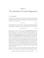
(2, −1)(−2, −1)
(0, 1)
ρ
1
ρ
2
Figure 13.1 The stationarity triangle for an AR(2) process
The result (13.08) makes it clear that ρ
1
and ρ
2
are not the autocorrelations of
an AR(2) process. Recall that, for an AR(1) process, the same ρ that appears
in the defining equation u
t
= ρu
t−1
+ ε
t
is also the correlation of u
t
and u
t−1
.
This simple result does not generalize to higher-order processes. Similarly,

the autocovariances and autocorrelations of u
t
and u
t−i
for i > 2 have a
more complicated form for AR processes of order greater than 1. They can,
however, be determined readily enough by using the Yule-Walker equations.
Thus, if we multiply both sides of equation (13.04) by u
t−i
for any i ≥ 2, and
take expectations, we obtain the equation
v
i
= ρ
1
v
i−1
+ ρ
2
v
i−2
.
Since
v
0
,
v
1
, and
v

2
are given by equations (13.08), this equation allows us to
solve recursively for any v
i
with i > 2.
Necessary conditions for the stationarity of the AR(2) process follow directly
from equations (13.08). The 3 ×3 covariance matrix


v
0
v
1
v
2
v
1
v
0
v
1
v
2
v
1
v
0


(13.09)

of any three consecutive elements of an AR(2) process must be a positive
definite matrix. Otherwise, the solution (13.08) to the first three Yule-Walker
equations, based on the hypothesis of stationarity, would make no sense. The
denominator D evidently must not vanish if this solution is to be finite. In
Exercise 12.3, readers are asked to show that the lines along which it vanishes
in the plane of ρ
1
and ρ
2
define the edges of a stationarity triangle such that
the matrix (13.09) is positive definite only in the interior of this triangle. The
stationarity triangle is shown in Figure 13.1.
Copyright
c
 1999, Russell Davidson and James G. MacKinnon
13.2 Autoregressive and Moving Average Processes 551
Moving Average Processes
A q
th
order moving average, or MA(q), process with a constant term can be
written as
y
t
= µ + α
0
ε
t
+ α
1
ε

t−1
+ . . . + α
q
ε
t−q
, (13.10)
where the ε
t
are white noise, and the coefficient α
0
is generally normalized
to 1 for purposes of identification. The expectation of the y
t
is readily seen
to be µ, and so we can write
u
t
≡ y
t
− µ = ε
t
+
q

j=1
α
j
ε
j
=


1 + α(L)

ε
t
,
where the polynomial α is defined by α(z) =

q
j=1
α
j
z
j
.
The autocovariances of an MA process are much easier to calculate than those
of an AR process. Since the ε
t
are white noise, and hence uncorrelated, the
variance of the u
t
is seen to be
Var(u
t
) = E(u
2
t
) = σ
2
ε


1 +
q

j=1
α
2
j

. (13.11)
Similarly, the j
th
order autocovariance is, for j > 0,
E(u
t
u
t−j
) =



σ
2
ε

α
j
+

q−j

i=1
α
j+i
α
i

for j < q,
σ
2
ε
α
j
for j = q, and
0 for j > q.
(13.12)
Using (13.12) and (13.11), we can calculate the autocorrelation ρ(j) between
y
t
and y
t−j
for j > 0.
1
We find that
ρ(j) =
α
j
+

q−j
i=1

α
j+i
α
i
1 +

q
i=1
α
2
i
for j ≤ q, ρ(j) = 0 otherwise, (13.13)
where it is understood that, for j = q, the numerator is just α
j
. The fact that
all of the autocorrelations are equal to 0 for j > q is sometimes convenient,
but it suggests that q may often have to be large if an MA(q) model is to be
satisfactory. Expression (13.13) also implies that q must be large if an MA(q)
model is to display any autocorrelation coefficients that are big in absolute
value. Recall from Section 7.6 that, for an MA(1) model, the largest possible
absolute value of ρ(1) is only 0.5.
1
The notation ρ is unfortunately in common use both for the parameters of an
AR process and for the autocorrelations of an AR or MA process. We therefore
distinguish between the parameter ρ
i
and the autocorrelation ρ(j).
Copyright
c
 1999, Russell Davidson and James G. MacKinnon

552 Methods for Stationary Time-Series Data
If we want to allow for nonzero autocorrelations at all lags, we have to allow
q to be infinite. This means replacing (13.10) by the infinite-order moving
average process
u
t
= ε
t
+
∞

i=1
α
i
ε
t−i
=

1 + α(L)

ε
t
, (13.14)
where α(L) is no longer a polynomial, but rather a (formal) infinite power
series in L. Of course, this MA(∞) process is impossible to estimate in
practice. Nevertheless, it is of theoretical interest, provided that
Var(u
t
) = σ
2

ε

1 +
∞

i=1
α
2
i

is a finite quantity. A necessary and sufficient condition for this to be the case
is that the coefficients α
j
are square summable, which means that
lim
q→∞
q

i=1
α
2
i
< ∞. (13.15)
We will implicitly assume that all the MA(∞) processes we encounter satisfy
condition (13.15).
Any stationary AR(p) process can be represented as an MA(∞) process. We
will not attempt to prove this fundamental result in general, but we can easily
show how it works in the case of a stationary AR(1) process. Such a process
can be written as
(1 −ρ

1
L)u
t
= ε
t
.
The natural way to solve this equation for u
t
as a function of ε
t
is to multiply
both sides by the inverse of 1 −ρ
1
L. The result is
u
t
= (1 −ρ
1
L)
−1
ε
t
. (13.16)
Formally, this is the solution we are seeking. But we need to explain what it
means to invert 1 − ρ
1
L.
In general, if A(L) and B(L) are power series in L, each including a constant
term independent of L that is not necessarily equal to 1, then B(L) is the
inverse of A(L) if B (L)A(L) = 1. Here the product B(L)A(L) is the infinite

power series in L obtained by formally multiplying together the power series
B(L) and A(L); see Exercise 13.5. The relation B(L)A(L) = 1 then requires
that the result of this multiplication should be a series with only one term,
the first. Moreover, this term, which corresponds to L
0
, must equal 1.
We will not consider general methods for inverting a polynomial in the lag
operator; see Hamilton (1994) or Hayashi (2000), among many others. In this
particular case, though, the solution turns out to be
(1 −ρ
1
L)
−1
= 1 + ρ
1
L + ρ
2
1
L
2
+ . . . . (13.17)
Copyright
c
 1999, Russell Davidson and James G. MacKinnon
13.2 Autoregressive and Moving Average Processes 553
To see this, note that ρ
1
L times the right-hand side of equation (13.17) is the
same series without the first term of 1. Thus, as required,
(1 −ρ

1
L)
−1
− ρ
1
L(1 −ρ
1
L)
−1
= (1 −ρ
1
L)(1 −ρ
1
L)
−1
= 1.
We can now use this result to solve equation (13.16). We find that
u
t
= ε
t
+ ρ
1
ε
t−1
+ ρ
2
1
ε
t−2

+ . . . . (13.18)
It is clear that (13.18) is a special case of the MA(∞) process (13.14), with
α
i
= ρ
i
1
for i = 0, . . . , ∞. Square summability of the α
i
is easy to check
provided that |ρ
1
| < 1.
In general, if we can write a stationary AR(p) process as

1 −ρ(L)

u
t
= ε
t
, (13.19)
where ρ(L) is a polynomial of degree p in the lag operator, then there exists
an MA(∞) process
u
t
=

1 + α(L)


ε
t
, (13.20)
where α(L) is an infinite series in L such that (1 −ρ(L))(1 + α(L)) = 1. This
result provides an alternative way to the Yule-Walker equations to calculate
the variance, autocovariances, and autocorrelations of an AR(p) process by
using equations (13.11), (13.12), and (13.13), after we have solved for α(L).
However, these methods make use of the theory of functions of a complex
variable, and so they are not elementary.
The close relationship between AR and MA processes goes both ways. If
(13.20) is an MA(q) process that is invertible, then there exists a stationary
AR(∞) process of the form (13.19) with

1 −ρ(L)

1 + α(L)

= 1.
The condition for a moving average process to be invertible is formally the
same as the condition for an autoregressive process to be stationary; see the
discussion around equation (7.36). We require that all the roots of the poly-
nomial equation 1 + α(z) = 0 must lie outside the unit circle. For an MA(1)
process, the invertibility condition is simply that |α
1
| < 1.
ARMA Processes
If our objective is to model the evolution of a time series as parsimoniously as
possible, it may well be desirable to employ a stochastic process that has both
autoregressive and moving average components. This is the autoregressive
moving average process, or ARMA process. In general, we can write an

ARMA(p, q) process with nonzero mean as

1 −ρ(L)

y
t
= γ +

1 + α(L)

ε
t
, (13.21)
Copyright
c
 1999, Russell Davidson and James G. MacKinnon
554 Methods for Stationary Time-Series Data
and a process with zero mean as

1 −ρ(L)

u
t
=

1 + α(L)

ε
t
, (13.22)

where ρ(L) and α(L) are, respectively, a p
th
order and a q
th
order polynomial
in the lag operator, neither of which includes a constant term. If the process is
stationary, the expectation of y
t
given by (13.21) is µ ≡ γ/

1 −ρ(1)

, just as
for the AR(p) process (13.01). Provided the autoregressive part is stationary
and the moving average part is invertible, an ARMA(p, q) process can always
be represented as either an MA(∞) or an AR(∞) process.
The most commonly encountered ARMA process is the ARMA(1,1) process,
which, when there is no constant term, has the form
u
t
= ρ
1
u
t−1
+ ε
t
+ α
1
ε
t−1

. (13.23)
This process has one autoregressive and one moving average parameter.
The Yule-Walker method can be extended to compute the autocovariances
of an ARMA process. We illustrate this for the ARMA(1, 1) case and invite
readers to generalize the procedure in Exercise 13.6. As before, we denote
the i
th
autocovariance by v
i
, and we let E(u
t
ε
t−i
) = w
i
, for i = 0, 1, . .
Note that E(u
t
ε
s
) = 0 for all s > t. If we multiply (13.23) by ε
t
and take
expectations, we see that w
0
= σ
2
ε
. If we then multiply (13.23) by ε
t−1

and
repeat the process, we find that w
1
= ρ
1
w
0
+ α
1
σ
2
ε
, from which we conclude
that w
1
= σ
2
ε
(ρ
1
+ α
1
). Although we do not need them at present, we note
that the w
i
for i > 1 can be found by multiplying (13.23) by ε
t−i
, which gives
the recursion w
i

= ρ
1
w
i−1
, with solution w
i
= σ
2
ε
ρ
i−1
1
(ρ
1
+ α
1
).
Next, we imitate the way in which the Yule-Walker equations are set up for
an AR process. Multiplying equation (13.23) first by u
t
and then by u
t−1
,
and subsequently taking expectations, gives
v
0
= ρ
1
v
1

+ w
0
+ α
1
w
1
= ρ
1
v
1
+ σ
2
ε
(1 + α
1
ρ
1
+ α
2
1
), and
v
1
= ρ
1
v
0
+ α
1
w

0
= ρ
1
v
0
+ α
1
σ
2
ε
,
where we have used the expressions for w
0
and w
1
given in the previous
paragraph. When these two equations are solved for v
0
and v
1
, they yield
v
0
= σ
2
ε
1 + 2ρ
1
α
1

+ α
2
1
1 −ρ
2
1
, and v
1
= σ
2
ε
ρ
1
+ ρ
2
1
α
1
+ ρ
1
α
2
1
+ α
1
1 −ρ
2
1
. (13.24)
Finally, multiplying equation (13.23) by u

t−i
for i > 1 and taking expectations
gives v
i
= ρ
1
v
i−1
, from which we conclude that
v
i
= σ
2
ε
ρ
i−1
1
(ρ
1
+ ρ
2
1
α
1
+ ρ
1
α
2
1
+ α

1
)
1 −ρ
2
1
. (13.25)
Copyright
c
 1999, Russell Davidson and James G. MacKinnon
13.2 Autoregressive and Moving Average Processes 555
Equation (13.25) provides all the autocovariances of an ARMA(1, 1) process.
Using it and the first of equations (13.24), we can derive the autocorrelations.
Autocorrelation Functions
As we have seen, the autocorrelation between u
t
and u
t−j
can be calculated
theoretically for any known stationary ARMA process. The autocorrelation
function, or ACF, expresses the autocorrelation as a function of the lag j for
j = 1, 2 . . If we have a sample y
t
, t = 1, . . . , n, from an ARMA process
of possibly unknown order, then the j
th
order autocorrelation ρ(j) can be
estimated by using the formula
ˆρ(j) =

Cov(y

t
, y
t−j
)

Var(y
t
)
, (13.26)
where

Cov(y
t
, y
t−j
) =
1
n −1
n

t=j+1
(y
t
− ¯y)(y
t−j
− ¯y), (13.27)
and

Var(y
t

) =
1
n −1
n

t=1
(y
t
− ¯y)
2
. (13.28)
In equations (13.27) and (13.28), ¯y is the mean of the y
t
. Of course, (13.28)
is just the special case of (13.27) in which j = 0. It may seem odd to divide
by n − 1 rather than by n − j − 1 in (13.27). However, if we did not use the
same denominator for every j, the estimated autocorrelation matrix would
not necessarily be positive definite. Because the denominator is the same, the
factors of 1/(n −1) cancel in the formula (13.26).
The empirical ACF, or sample ACF, expresses the ˆρ(j), defined in equation
(13.26), as a function of the lag j. Graphing the sample ACF provides a
convenient way to see what the pattern of serial dependence in any observed
time series looks like, and it may help to suggest what sort of stochastic
process would provide a good way to model the data. For example, if the
data were generated by an MA(1) process, we would expect that ˆρ(1) would
be an estimate of α
1
and all the other ˆρ(j) would be approximately equal to
zero. If the data were generated by an AR(1) process with ρ
1

> 0, we would
expect that ˆρ(1) would be an estimate of ρ
1
and would be relatively large, the
next few ˆρ(j) would be progressively smaller, and the ones for large j would
be approximately equal to zero. A graph of the sample ACF is sometimes
called a correlogram; see Exercise 13.15.
The partial autocorrelation function, or PACF, is another way to characterize
the relationship between y
t
and its lagged values. The partial autocorrelation
coefficient of order j is defined as the true value of the coefficient ρ
(j)
j
in the
linear regression
y
t
= γ
(j)
+ ρ
(j)
1
y
t−1
+ . . . + ρ
(j)
j
y
t−j

+ ε
t
, (13.29)
Copyright
c
 1999, Russell Davidson and James G. MacKinnon
556 Methods for Stationary Time-Series Data
or, equivalently, in the minimization problem
min
γ
(j)
, ρ
(j)
i
E

y
t
− γ
(j)
−
j

i=1
ρ
(j)
i
y
t−i


2
. (13.30)
The superscript “(j)” appears on all the coefficients in regression (13.29) to
make it plain that all the coefficients, not just the last one, are functions of j,
the number of lags. We can calculate the empirical PACF, or sample PACF,
up to order J by running regression (13.29) for j = 1, . . . , J and retaining
only the estimate ˆρ
(j)
j
for each j. Just as a graph of the sample ACF may
help to suggest what sort of stochastic process would provide a good way to
model the data, so a graph of the sample PACF, interpreted properly, may
do the same. For example, if the data were generated by an AR(2) process,
we would expect the first two partial autocorrelations to be relatively large,
and all the remaining ones to be insignificantly different from zero.
13.3 Estimating AR, MA, and ARMA Models
All of the time-series models that we have discussed so far are special cases
of an ARMA(p, q) model with a constant term, which can be written as
y
t
= γ +
p

i=1
ρ
i
y
t−i
+ ε
t

+
q

j=1
α
j
ε
t−j
, (13.31)
where the ε
t
are assumed to be white noise. There are p + q +1 parameters to
estimate in the model (13.31): the ρ
i
, for i = 1, . . . , p, the α
j
, for j = 1, . . . , q,
and γ. Recall that γ is not the unconditional expectation of y
t
unless all of
the ρ
i
are zero.
For our present purposes, it is perfectly convenient to work with models that
allow y
t
to depend on exogenous explanatory variables and are therefore even
more general than (13.31). Such models are sometimes referred to as ARMAX
models. The ‘X’ indicates that y
t

depends on a row vector X
t
of exogenous
variables as well as on its own lagged values. An ARMAX(
p, q
) model takes
the form
y
t
= X
t
β + u
t
, u
t
∼ ARMA(p, q), E(u
t
) = 0, (13.32)
where X
t
β is the mean of y
t
conditional on X
t
but not conditional on lagged
values of y
t
. The ARMA model (13.31) can evidently be recast in the form
of the ARMAX model (13.32); see Exercise 13.13.
Estimation of AR Models

We have already studied a variety of ways of estimating the model (13.32)
when u
t
follows an AR(1) process. In Chapter 7, we discussed three estimation
Copyright
c
 1999, Russell Davidson and James G. MacKinnon
13.3 Estimating AR, MA, and ARMA Models 557
methods. The first was estimation by a nonlinear regression, in which the
first observation is dropped from the sample. The second was estimation by
feasible GLS, possibly iterated, in which the first observation can be taken
into account. The third was estimation by the GNR that corresponds to
the nonlinear regression with an extra artificial observation corresponding to
the first observation. It turned out that estimation by iterated feasible GLS
and by this extended artificial regression, both taking the first observation
into account, yield the same estimates. Then, in Chapter 10, we discussed
estimation by maximum likelihood, and, in Exercise 10.21, we showed how to
extend the GNR by yet another artificial observation in such a way that it
provides the ML estimates if convergence is achieved.
Similar estimation methods exist for models in which the error terms follow
an AR(p) process with p > 1. The easiest method is just to drop the first p
observations and estimate the nonlinear regression model
y
t
= X
t
β +
p

i=1

ρ
i
(y
t−i
− X
t−i
β) + ε
t
by nonlinear least squares. If this is a pure time-series model for which
X
t
β = β, then this is equivalent to OLS estimation of the model
y
t
= γ +
p

i=1
ρ
i
y
t−i
+ ε
t
,
where the relationship between γ and β is derived in Exercise 13.13. This
approach is the simplest and most widely used for pure autoregressive models.
It has the advantage that, although the ρ
i
(but not their estimates) must

satisfy the necessary condition for stationarity, the error terms u
t
need not
be stationary. This issue was mentioned in Section 7.8, in the context of the
AR(1) model, where it was seen that the variance of the first error term u
1
must satisfy a certain condition for u
t
to be stationary.
Maximum Likelihood Estimation
If we are prepared to assume that u
t
is indeed stationary, it is desirable not
to lose the information in the first p observations. The most convenient way
to achieve this goal is to use maximum likelihood under the assumption that
the white noise process ε
t
is normal. In addition to using more information,
maximum likelihood has the advantage that the estimates of the ρ
j
are auto-
matically constrained to satisfy the stationarity conditions.
For any ARMA(p, q) process in the error terms u
t
, the assumption that the ε
t
are normally distributed implies that the u
t
are normally distributed, and so
also the dependent variable y

t
, conditional on the explanatory variables. For
an observed sample of size n from the ARMAX model (13.32), let y denote
the n vector of which the elements are y
1
, . . . , y
n
. The expectation of y
conditional on the explanatory variables is Xβ, where X is the n ×k matrix
Copyright
c
 1999, Russell Davidson and James G. MacKinnon
558 Methods for Stationary Time-Series Data
with typical row X
t
. Let Ω denote the autocovariance matrix of the vector y.
This matrix can be written as
Ω =






v
0
v
1
v
2

. . . v
n−1
v
1
v
0
v
1
. . . v
n−2
v
2
v
1
v
0
. . . v
n−3
.
.
.
.
.
.
.
.
.
.
.
.

.
.
.
v
n−1
v
n−2
v
n−3
. . . v
0






, (13.33)
where, as before, v
i
is the stationary covariance of u
t
and u
t−i
, and v
0
is
the stationary variance of the u
t
. Then, using expression (12.121) for the

multivariate normal density, we see that the log of the joint density of the
observed sample is
−
n
−
2
log 2π −
1
−
2
log |Ω| −
1
−
2
(y − Xβ)

Ω
−1
(y − Xβ). (13.34)
In order to construct the loglikelihood function for the ARMAX model (13.32),
the v
i
must be expressed as functions of the parameters ρ
i
and α
j
of the
ARMA(p, q) process that generates the error terms. Doing this allows us to
replace Ω in the log density (13.34) by a matrix function of these parameters.
Unfortunately, a loglikelihood function in the form of (13.34) is difficult to

work with, because of the presence of the n × n matrix Ω. Most of the
difficulty disappears if we can find an upper-triangular matrix Ψ such that
Ψ Ψ

= Ω
−1
, as was necessary when, in Section 7.8, we wished to estimate by
feasible GLS a model like (13.32) with AR(1) errors. It then becomes possible
to decompose expression (13.34) into a sum of contributions that are easier
to work with than (13.34) itself.
If the errors are generated by an AR(p) process, with no MA component, then
such a matrix Ψ is relatively easy to find, as we will illustrate in a moment
for the AR(2) case. However, if an MA component is present, matters are
more difficult. Even for MA(1) errors, the algebra is quite complicated — see
Hamilton (1994, Chapter 5) for a convincing demonstration of this fact. For
general ARMA(p, q) processes, the algebra is quite intractable. In such cases,
a technique called the Kalman filter can be used to evaluate the successive con-
tributions to the loglikelihood for given parameter values, and can thus serve
as the basis of an algorithm for maximizing the loglikelihood. This technique,
to which Hamilton (1994, Chapter 13) provides an accessible introduction, is
unfortunately beyond the scope of this book.
We now turn our attention to the case in which the errors follow an AR(2)
process. In Section 7.8, we constructed a matrix Ψ corresponding to the sta-
tionary covariance matrix of an AR(1) process by finding n linear combina-
tions of the error terms u
t
that were homoskedastic and serially uncorrelated.
We perform a similar exercise for AR(2) errors here. This will show how to
set about the necessary algebra for more general AR(p) processes.
Copyright

c
 1999, Russell Davidson and James G. MacKinnon
13.3 Estimating AR, MA, and ARMA Models 559
Errors generated by an AR(2) process satisfy equation (13.04). Therefore, for
t ≥ 3, we can solve for ε
t
to obtain
ε
t
= u
t
− ρ
1
u
t−1
− ρ
2
u
t−2
, t = 3, . . . , n. (13.35)
Under the normality assumption, the fact that the ε
t
are white noise means
that they are mutually independent. Thus observations 3 through n make
contributions to the loglikelihood of the form

t
(y
t
, β, ρ

1
, ρ
2
, σ
ε
) =
−
1
−
2
log 2π − log σ
ε
−
1
2σ
2
ε

u
t
(β) − ρ
1
u
t−1
(β) − ρ
2
u
t−2
(β)


2
,
(13.36)
where y
t
is the vector that consists of y
1
through y
t
, u
t
(β) ≡ y
t
− X
t
β, and
σ
2
ε
is as usual the variance of the ε
t
. The contribution (13.36) is analogous to
the contribution (10.85) for the AR(1) case.
The variance of the first error term, u
1
, is just the stationary variance v
0
given
by (13.08). We can therefore define ε
1

as σ
ε
u
1
/
√
v
0
, that is,
ε
1
=

D
1 −ρ
2

1/2
u
1
, (13.37)
where D was defined just after equations (13.08). By construction, ε
1
has the
same variance σ
2
ε
as the ε
t
for t ≥ 3. Since the ε

t
are innovations, it follows
that, for t > 1, ε
t
is independent of u
1
, and hence of ε
1
. For the loglikelihood
contribution from observation 1, we therefore take the log density of ε
1
, plus
a Jacobian term which is the log of the derivative of ε
1
with respect to u
1
.
The result is readily seen to be

1
(y
1
, β, ρ
1
, ρ
2
, σ
ε
) =
−

1
−
2
log 2π − log σ
ε
+
1
−
2
log
D
1 −ρ
2
−
D
2σ
2
ε
(1 −ρ
2
)
u
2
1
(β).
(13.38)
Finding a suitable expression for ε
2
is a little trickier. What we seek is a linear
combination of u

1
and u
2
that has variance σ
2
ε
and is independent of u
1
. By
construction, any such linear combination is independent of the ε
t
for t > 2.
A little algebra shows that the appropriate linear combination is
σ
ε

v
0
v
2
0
− v
2
1

1/2

u
2
−

v
1
v
0
u
1

.
Use of the explicit expressions for v
0
and v
1
given in equations (13.08) then
shows that
ε
2
= (1 −ρ
2
2
)
1/2

u
2
−
ρ
1
1 −ρ
2
u

1

, (13.39)
Copyright
c
 1999, Russell Davidson and James G. MacKinnon
560 Methods for Stationary Time-Series Data
as readers are invited to check in Exercise 13.9. The derivative of ε
2
with
respect to u
2
is (1 −ρ
2
2
)
1/2
, and so the contribution to the loglikelihood from
observation 2 can be written as

2
(y
2
, β, ρ
1
, ρ
2
, σ
ε
) = −

1
−
2
log 2π − log σ
ε
+
1
−
2
log(1 −ρ
2
2
)
−
1 −ρ
2
2
2σ
2
ε

u
2
(β) −
ρ
1
1 −ρ
2
u
1

(β)

2
.
(13.40)
Summing the contributions (13.36), (13.38), and (13.40) gives the loglikeli-
hood function for the entire sample. It may then be maximized with respect
to β, ρ
1
, ρ
2
, and σ
2
ε
by standard numerical methods.
Exercise 13.10 asks readers to check that the n×n matrix Ψ defined implicitly
by the relation Ψ

u = ε, where the elements of ε are defined by (13.35),
(13.37), and (13.39), is indeed upper triangular and such that Ψ Ψ

is equal
to 1/σ
2
ε
times the inverse of the covariance matrix (13.33) for the v
i
that
correspond to an AR(2) process.
Estimation of MA and ARMA Models

Just why moving average and ARMA models are more difficult to estimate
than pure autoregressive models is apparent if we consider the MA(1) model
y
t
= µ + ε
t
− α
1
ε
t−1
, (13.41)
where for simplicity the only explanatory variable is a constant, and we have
changed the sign of α
1
. For the first three observations, if we substitute
recursively for ε
t−1
, equation (13.41) can be written as
y
1
= µ −α
1
ε
0
+ ε
1
,
y
2
= (1 + α

1
)µ −α
1
y
1
− α
2
1
ε
0
+ ε
2
,
y
3
= (1 + α
1
+ α
2
1
)µ −α
1
y
2
− α
2
1
y
1
− α

3
1
ε
0
+ ε
3
.
It is not difficult to see that, for arbitrary t, this becomes
y
t
=

t−1

s=0
α
s
1

µ −
t−1

s=1
α
s
1
y
t−s
− α
t

1
ε
0
+ ε
t
. (13.42)
Were it not for the presence of the unobserved ε
0
, equation (13.42) would be
a nonlinear regression model, alb eit a rather complicated one in which the
form of the regression function depends explicitly on t.
This fact can be used to develop tractable methods for estimating a model
where the errors have an MA component without going to the trouble of set-
ting up the complicated loglikelihood. The estimates are not equal to ML es-
timates, and are in general less efficient, although in some cases they are
Copyright
c
 1999, Russell Davidson and James G. MacKinnon
13.3 Estimating AR, MA, and ARMA Models 561
asymptotically equivalent. The simplest approach, which is sometimes rather
misleadingly called conditional least squares, is just to assume that any unob-
served pre-sample innovations, such as ε
0
, are equal to 0, an assumption that
is harmless asymptotically. A more sophisticated approach is to “backcast”
the pre-sample innovations from initial estimates of the other parameters and
then run the nonlinear regression (13.42) conditional on the backcasts, that is,
the backward forecasts. Yet another approach is to treat the unobserved in-
novations as parameters to be estimated jointly by maximum likelihood with
the parameters of the MA process and those of the regression function.

Alternative statistical packages use a number of different methods for esti-
mating mo dels with ARMA errors, and they may therefore yield different
estimates; see Newbold, Agiakloglou, and Miller (1994) for a more detailed
account. Moreover, even if they provide the same estimates, different pack-
ages may well provide different standard errors. In the case of ML estimation,
for example, these may be based on the empirical Hessian estimator (10.42),
the OPG estimator (10.44), or the sandwich estimator (10.45), among others.
If the innovations are heteroskedastic, only the sandwich estimator is valid.
A more detailed discussion of standard methods for estimating AR, MA, and
ARMA models is beyond the scope of this book. Detailed treatments may
be found in Box, Jenkins, and Reinsel (1994, Chapter 7), Hamilton (1994,
Chapter 5), and Fuller (1995, Chapter 8), among others.
Indirect Inference
There is another approach to estimating ARMA models, which is unlikely to
be used by statistical packages but is worthy of attention if the available sam-
ple is not too small. It is an application of the method of indirect inference,
which was developed by Smith (1993) and Gouri´eroux, Monfort, and Renault
(1993). The idea is that, when a model is difficult to estimate, there may be
an auxiliary model that is not too different from the model of interest but
is much easier to estimate. For any two such models, there must exist so-
called binding functions that relate the parameters of the model of interest to
those of the auxiliary model. The idea of indirect inference is to estimate the
parameters of interest from the parameter estimates of the auxiliary model
by using the relationships given by the binding functions.
Because pure AR models are easy to estimate and can be used as auxiliary
models, it is natural to use this approach with models that have an MA
component. For simplicity, suppose the model of interest is the pure time-
series MA(1) model (13.41), and the auxiliary model is the AR(1) model
y
t

= γ + ρy
t−1
+ u
t
, (13.43)
which we estimate by OLS to obtain estimates ˆγ and ˆρ. Let us define the
elementary zero function u
t
(γ, ρ) as y
t
− γ − ρy
t−1
. Then the estimating
Copyright
c
 1999, Russell Davidson and James G. MacKinnon
562 Methods for Stationary Time-Series Data
equations satisfied by ˆγ and ˆρ are
n

t=2
u
t
(γ, ρ) = 0 and
n

t=2
y
t−1
u

t
(γ, ρ) = 0. (13.44)
If y
t
is indeed generated by (13.41) for particular values of µ and α
1
, then we
may define the pseudo-true values of the parameters γ and ρ of the auxiliary
model (13.43) as those values for which the expectations of the left-hand sides
of equations (13.44) are zero. These equations can thus be interpreted as
correctly specified, albeit inefficient, estimating equations for the pseudo-true
values. The theory of Section 9.5 then shows that ˆγ and ˆρ are consistent for
the pseudo-true values and asymptotically normal, with asymptotic covariance
matrix given by a version of the sandwich matrix (9.67).
The pseudo-true values can be calculated as follows. Replacing y
t
and y
t−1
in the definition of u
t
(γ, ρ) by the expressions given by (13.41), we see that
u
t
(γ, ρ) = (1 −ρ )µ −γ + ε
t
− (α
1
+ ρ)ε
t−1
+ α

1
ρε
t−2
. (13.45)
The expectation of the right-hand side of this equation is just (1 − ρ) µ − γ.
Similarly, the expectation of y
t−1
u
t
(γ, ρ) can be seen to b e
µ

(1 −ρ)µ −γ) −σ
2
ε
(α
1
+ ρ) −σ
2
ε
α
2
1
ρ.
Equating these expectations to zero shows us that the pseudo-true values are
γ =
µ(1 + α
1
+ α
2

1
)
1 + α
2
1
and ρ =
−α
1
1 + α
2
1
(13.46)
in terms of the true parameters µ and α
1
.
Equations (13.46) express the binding functions that link the parameters of
model (13.41) to those of the auxiliary model (13.43). The indirect estimates
ˆµ and ˆα
1
are obtained by solving these equations with γ and ρ replaced by ˆγ
and ˆρ. Note that, since the second equation of (13.46) is a quadratic equation
for α
1
in terms of ρ, there are in general two solutions for α
1
, which may be
complex. See Exercise 13.11 for further elucidation of this point.
In order to estimate the covariance matrix of ˆµ and ˆα
1
, we must first estimate

the covariance matrix of ˆγ and ˆρ. Let us define the n ×2 matrix Z as [ι y
−1
],
that is, a matrix of which the first column is a vector of 1s and the second the
vector of the y
t
lagged. Then, since the Jacobian of the zero functions u
t
(γ, ρ)
is just −Z, it is easy to see that the covariance matrix (9.67) becomes
plim
n→∞
1
−
n
(Z

Z)
−1
Z

ΩZ(Z

Z)
−1
, (13.47)
where Ω is the covariance matrix of the error terms u
t
, which are given by
the u

t
(γ, ρ) evaluated at the pseudo-true values. If we drop the probability
Copyright
c
 1999, Russell Davidson and James G. MacKinnon
13.3 Estimating AR, MA, and ARMA Models 563
limit and the factor of n
−1
in expression (13.47) and replace Ω by a suitable
estimate, we obtain an estimate of the covariance matrix of ˆγ and ˆρ. Instead
of estimating Ω directly, it is convenient to employ a HAC estimator of the
middle factor of expression (13.47).
2
Since, as can be seen from equation
(13.45), the u
t
have nonzero autocovariances only up to order 2, it is natural
in this case to use the Hansen-White estimator (9.37) with lag truncation
parameter set equal to 2. Finally, an estimate of the covariance matrix of
ˆµ and ˆα
1
can be obtained from the one for ˆγ and ˆρ by the delta method
(Section 5.6) using the relation (13.46) between the true and pseudo-true
parameters.
In this example, indirect inference is particularly simple because the auxiliary
model (13.43) has just as many parameters as the model of interest (13.41).
However, this will rarely be the case. We saw in Section 13.2 that a finite-order
MA or ARMA process can always be represented by an AR(∞) process. This
suggests that, when estimating an MA or ARMA model, we should use as an
auxiliary model an AR(p) model with p substantially greater than the number

of parameters in the model of interest. See Zinde-Walsh and Galbraith (1994,
1997) for implementations of this approach.
Clearly, indirect inference is impossible if the auxiliary model has fewer para-
meters than the model of interest. If, as is commonly the case, it has more,
then the parameters of the model of interest are overidentified. This means
that we cannot just solve for them from the estimates of the auxiliary model.
Instead, we need to minimize a suitable criterion function, so as to make the
estimates of the auxiliary model as close as possible, in the appropriate sense,
to the values implied by the parameter estimates of the model of interest. In
the next paragraph, we explain how to do this in a very general setting.
Let the estimates of the pseudo-true parameters be an l vector
ˆ
β, let the
parameters of the model of interest be a k vector θ, and let the binding
functions be an l vector b(θ), with l > k. Then the indirect estimator of θ is
obtained by minimizing the quadratic form

ˆ
β − b(θ)


ˆ
Σ
−1

ˆ
β − b(θ)

(13.48)
with respect to θ, where

ˆ
Σ is a consistent estimate of the l × l covariance
matrix of
ˆ
β. Minimizing this quadratic form minimizes the length of the
vector
ˆ
β −b(θ) after that vector has been transformed so that its covariance
matrix is approximately the identity matrix.
Expression (13.48) looks very much like a criterion function for efficient GMM
estimation. Not surprisingly, it can b e shown that, under suitable regularity
2
In this special case, an expression for Ω as a function of α, ρ, and σ
2
ε
can be
obtained from equation (13.45), so that we can estimate Ω as a function of
consistent estimates of those parameters. In most cases, however, it will be
necessary to use a HAC estimator.
Copyright
c
 1999, Russell Davidson and James G. MacKinnon
564 Methods for Stationary Time-Series Data
conditions, the minimized value of this criterion function is asymptotically
distributed as χ
2
(l−k). This provides a simple way to test the overidentifying
restrictions that must hold if the model of interest actually generated the data.
As with efficient GMM estimation, tests of restrictions on the vector θ can
be based on the difference between the restricted and unrestricted values of

expression (13.48).
In many applications, including general ARMA processes, it can be difficult or
impossible to find tractable analytic expressions for the binding functions. In
that case, they may be estimated by simulation. This works well if it is easy
to draw simulated samples from DGPs in the model of interest, and also easy
to estimate the auxiliary model. Simulations are then carried out as follows.
In order to evaluate the criterion function (13.48) at a parameter vector θ, we
draw S independent simulated data sets from the DGP characterized by θ,
and for each of them we compute the estimate β
∗
s
(θ) of the parameters of the
auxiliary model. The binding functions are then estimated by
b
∗
(θ) =
1
S
S

s=1
β
∗
s
(θ).
We then use b
∗
(θ) in place of b(θ) when we evaluate the criterion function
(13.48). As with the method of simulated moments (Section 9.6), the same
random numbers should be used to compute β

∗
s
for each given s and for all θ.
Much more detailed discussions of indirect inference can be found in Smith
(1993) and Gouri´eroux, Monfort, and Renault (1993).
Simulating ARMA Models
Simulating data from an MA(q) process is trivially easy. For a sample of
size n, one generates white-noise innovations ε
t
for t = −q + 1, . . . , 0, . . . , n,
most commonly, but not necessarily, from the normal distribution. Then, for
t = 1, . . . , n, the simulated data are given by
u
∗
t
= ε
t
+
q

j=1
α
j
ε
t−j
.
There is no need to worry about missing pre-sample innovations in the context
of simulation, because they are simulated along with the other innovations.
Simulating data from an AR(p) process is not quite so easy, because of the
initial observations. Recursive simulation can be used for all but the first p

observations, using the equation
u
∗
t
=
p

i=1
ρ
i
u
∗
t−i
+ ε
t
. (13.49)
For an AR(1) process, the first simulated observation u
∗
1
can be drawn from
the stationary distribution of the process, by which we mean the unconditional
Copyright
c
 1999, Russell Davidson and James G. MacKinnon
13.4 Single-Equation Dynamic Models 565
distribution of u
t
. This distribution has mean zero and variance σ
2
ε

/(1 −ρ
2
1
).
The remaining observations are then generated recursively. When p > 1,
the first p observations must be drawn from the stationary distribution of p
consecutive elements of the AR(p) series. This distribution has mean vector
zero and covariance matrix Ω given by expression (13.33) with n = p. Once
the specific form of this covariance matrix has been determined, perhaps by
solving the Yule-Walker equations, and Ω has been evaluated for the spe-
cific values of the ρ
i
, a p × p lower-triangular matrix A can be found such
that AA

= Ω; see the discussion of the multivariate normal distribution in
Section 4.3. We then generate ε
p
as a p vector of white noise innovations
and construct the p vector u
∗
p
of the first p observations as u
∗
p
= Aε
p
. The
remaining observations are then generated recursively.
Since it may take considerable effort to find Ω, a simpler technique is often

used. One starts the recursion (13.49) for a large negative value of t with
essentially arbitrary starting values, often zero. By making the starting value
of t far enough in the past, the joint distribution of u
∗
1
through u
∗
p
can be
made arbitrarily close to the stationary distribution. The values of u
∗
t
for
nonpositive t are then discarded.
Starting the recursion far in the past also works with an ARMA(p, q) model.
However, at least for simple models, we can exploit the covariances computed
by the extension of the Yule-Walker method discussed in Section 13.2. The
process (13.22) can be written explicitly as
u
∗
t
=
p

i=1
ρ
i
u
∗
t−i

+ ε
t
+
q

j=1
α
j
ε
t−j
. (13.50)
In order to be able to compute the u
∗
t
recursively, we need starting values for
u
∗
1
, . . . , u
∗
p
and ε
p−q+1
, . . . , ε
p
. Given these, we can compute u
∗
p+1
by drawing
the innovation ε

p+1
and using equation (13.50) for t = p + 1, . . . , n. The
starting values can be drawn from the joint stationary distribution character-
ized by the autocovariances v
i
and covariances w
j
discussed in the previous
section. In Exercise 13.12, readers are asked to find this distribution for the
relatively simple ARMA(1, 1) case.
13.4 Single-Equation Dynamic Models
Economists often wish to model the relationship between the current value
of a dependent variable y
t
, the current and lagged values of one or more
independent variables, and, quite possibly, lagged values of y
t
itself. This sort
of model can be motivated in many ways. Perhaps it takes time for economic
agents to perceive that the independent variables have changed, or perhaps it
is costly for them to adjust their behavior. In this section, we briefly discuss
a number of models of this type. For notational simplicity, we assume that
Copyright
c
 1999, Russell Davidson and James G. MacKinnon
566 Methods for Stationary Time-Series Data
there is only one independent variable, denoted x
t
. In practice, of course,
there is usually more than one such variable, but it will be obvious how to

extend the models we discuss to handle this more general case.
Distributed Lag Models
When a dependent variable depends on current and lagged values of x
t
, but
not on lagged values of itself, we have what is called a distributed lag model.
When there is only one independent variable, plus a constant term, such a
model can be written as
y
t
= δ +
q

j=0
β
j
x
t−j
+ u
t
, u
t
∼ IID(0, σ
2
), (13.51)
in which y
t
depends on the current value of x
t
and on q lagged values. The

constant term δ and the coefficients β
j
are to be estimated.
In many cases, x
t
is positively correlated with some or all of the lagged values
x
t−j
for j ≥ 1. In consequence, the OLS estimates of the β
j
in equation
(13.51) may be quite imprecise. However, this is generally not a problem if
we are merely interested in the long-run impact of changes in the independent
variable. This long-run impact is
γ ≡
q

j=0
β
j
=
q

j=0
∂y
t
∂x
t−j
. (13.52)
We can estimate (13.51) and then calculate the estimate ˆγ using (13.52), or

we can obtain ˆγ directly by reparametrizing regression (13.51) as
y
t
= δ + γx
t
+
q

j=1
β
j
(x
t−j
− x
t
) + u
t
. (13.53)
The advantage of this reparametrization is that the standard error of ˆγ is
immediately available from the regression output.
In Section 3.4, we derived an expression for the variance of a weighted sum
of parameter estimates. Expression (3.33), which can be written in a more
intuitive fashion as (3.68), can be applied directly to ˆγ, which is an unweighted
sum. If we do so, we find that
Var(ˆγ) = ι

Var(
ˆ
β)ι =
q


j=0
Var(
ˆ
β
j
) + 2
q

j=1
j−1

k=0
Cov(
ˆ
β
j
,
ˆ
β
k
), (13.54)
where the smallest value of j in the double summation is 1 rather than 0,
because no valid value of k exists for j = 0. When x
t−j
is positively correlated
with x
t−k
for all j = k, the covariance terms in (13.54) are generally all
negative. When the correlations are large, these covariance terms can often

be large in absolute value, so much so that Var(ˆγ) may be smaller than the
variance of
ˆ
β
j
for some or all j. If we are interested in the long-run impact of
x
t
on y
t
, it is therefore perfectly sensible just to estimate equation (13.53).
Copyright
c
 1999, Russell Davidson and James G. MacKinnon
13.4 Single-Equation Dynamic Models 567
The Partial Adjustment Model
One popular alternative to distributed lag models like (13.51) is the partial
adjustment model, which dates back at least to Nerlove (1958). Suppose that
the desired level of an economic variable y
t
is y
◦
t
. This desired level is assumed
to depend on a vector of exogenous variables X
t
according to
y
◦
t

= X
t
β
◦
+ e
t
, e
t
∼ IID(0, σ
2
e
). (13.55)
Because of adjustment costs, y
t
is not equal to y
◦
t
in every period. Instead, it
is assumed to adjust toward y
◦
t
according to the equation
y
t
− y
t−1
= (1 −δ)(y
◦
t
− y

t−1
) + v
t
, v
t
∼ IID(0, σ
2
v
), (13.56)
where δ is an adjustment parameter that is assumed to be positive and strictly
less than 1. Solving (13.55) and (13.56) for y
t
, we find that
y
t
= y
t−1
− (1 − δ)y
t−1
+ (1 − δ)X
t
β
◦
+ (1 − δ)e
t
+ v
t
= X
t
β + δy

t−1
+ u
t
,
(13.57)
where β ≡ (1 − δ)β
◦
and u
t
≡ (1 − δ)e
t
+ v
t
. Thus the partial adjustment
model leads to a linear regression of y
t
on X
t
and y
t−1
. The coefficient of
y
t−1
is the adjustment parameter, and estimates of β
◦
can be obtained from
the OLS estimates of β and δ. This model does not make sense if δ < 0 or if
δ ≥ 1. Moreover, when δ is close to 1, the implied speed of adjustment may
be implausibly slow.
Equation (13.57) can be solved for y

t
as a function of current and lagged
values of X
t
and u
t
. Under the assumption that |δ| < 1, we find that
y
t
=
∞

j=0
δ
j
X
t−j
β +
∞

j=0
δ
j
u
t−j
.
Thus we see that the partial adjustment model implies a particular form of
distributed lag. However, in contrast to the model (13.51), y
t
now depends on

lagged values of the error terms u
t
as well as on lagged values of the exogenous
variables X
t
. This makes sense in many cases. If the regressors affect y
t
via a
distributed lag, and if the error terms reflect the combined influence of other
regressors that have been omitted, then it is surely plausible that the omitted
regressors would also affect y
t
via a distributed lag. However, the restriction
that the same distributed lag coefficients should apply to all the regressors
and to the error terms may be excessively strong in many cases.
The partial adjustment model is only one of many economic models that can
be used to justify the inclusion of one or more lags of the dependent variables
in regression functions. Others are discussed in Dhrymes (1971) and Hendry,
Pagan, and Sargan (1984). We now consider a general family of regression
models that include lagged dependent and lagged independent variables.
Copyright
c
 1999, Russell Davidson and James G. MacKinnon
568 Methods for Stationary Time-Series Data
Autoregressive Distributed Lag Models
For simplicity of notation, we will continue to discuss only models with a
single independent variable, x
t
. In this case, an autoregressive distributed
lag, or ADL, model can be written as

y
t
= β
0
+
p

i=1
β
i
y
t−i
+
q

j=0
γ
j
x
t−j
+ u
t
, u
t
∼ IID(0, σ
2
). (13.58)
Because there are p lags on y
t
and q lags on x

t
, this is sometimes called an
ADL(p, q) model.
A widely encountered special case of (13.58) is the ADL(1, 1) model
y
t
= β
0
+ β
1
y
t−1
+ γ
0
x
t
+ γ
1
x
t−1
+ u
t
. (13.59)
Because most results that are true for the ADL(1, 1) model are also true, with
obvious modifications, for the more general ADL(p, q) model, we will largely
confine our discussion to this special case.
Although the ADL(1, 1) model is quite simple, many commonly encountered
models are special cases of it. When β
1
= γ

1
= 0, we have a static regression
model with IID errors; when γ
0
= γ
1
= 0, we have a univariate AR(1) model;
when γ
1
= 0, we have a partial adjustment model; when γ
1
= −β
1
γ
0
, we have
a static regression model with AR(1) errors; and when β
1
= 1 and γ
1
= −γ
0
,
we have a model in first differences that can be written as
∆y
t
= β
0
+ γ
0

∆x
t
+ u
t
.
Before we accept any of these special cases, it makes sense to test them
against (13.59). This can be done by means of asymptotic t or F tests, which
it may be wise to bootstrap when the sample size is not large.
It is usually desirable to impose the condition that |β
1
| < 1 in (13.59). Strictly
speaking, this is not a stationarity condition, since we cannot expect y
t
to be
stationary without imposing further conditions on the explanatory variable x
t
.
However, it is easy to see that, if this condition is violated, the dependent
variable y
t
exhibits explosive behavior. If the condition is satisfied, there may
exist a long-run equilibrium relationship between y
t
and x
t
, which can be used
to develop a particularly interesting reparametrization of (13.59).
Suppose there exists an equilibrium value x
◦
to which x

t
would converge as
t → ∞ in the absence of shocks. Then, in the absence of the error terms u
t
,
y
t
would converge to a steady-state long-run equilibrium value y
◦
such that
y
◦
= β
0
+ β
1
y
◦
+ (γ
0
+ γ
1
)x
◦
.
Solving this equation for y
◦
as a function of x
◦
yields

y
◦
=
β
0
1 −β
1
+
γ
0
+ γ
1
1 −β
1
x
◦
=
β
0
1 −β
1
+ λx
◦
, (13.60)
Copyright
c
 1999, Russell Davidson and James G. MacKinnon
13.4 Single-Equation Dynamic Models 569
where
λ ≡

γ
0
+ γ
1
1 −β
1
. (13.61)
This is the long-run derivative of y
◦
with respect to x
◦
, and it is an elasticity
if both series are in logarithms. An estimate of λ can be computed directly
from the estimates of the parameters of (13.59). Note that the result (13.60)
and the definition (13.61) make sense only if the condition |β
1
| < 1 is satisfied.
Because it is so general, the ADL(p, q) model is a good place to start when
attempting to specify a dynamic regression model. In many cases, setting
p = q = 1 will be sufficiently general, but with quarterly data it may be wise
to start with p = q = 4. Of course, we very often want to impose restrictions
on such a model. Depending on how we write the model, different restrictions
may naturally suggest themselves. These can b e tested in the usual way by
means of asymptotic F and t tests, which may be bootstrapped to improve
their finite-sample properties.
Error-Correction Models
It is a straightforward exercise to check that the ADL(1, 1) model of equation
(13.59) can be rewritten as
∆y
t

= β
0
+ (β
1
− 1)(y
t−1
− λx
t−1
) + γ
0
∆x
t
+ u
t
, (13.62)
where λ was defined in (13.61). Equation (13.62) is called an error-correction
model. It expresses the ADL(1, 1) model in terms of an error-correction
mechanism; both the model and mechanism are often abbreviated to ECM.
3
Although the model (13.62) appears to be nonlinear, it is really just a repara-
metrization of the linear model (13.59). If the latter is estimated by OLS, an
appropriate GNR can be used to obtain the covariance matrix of the estimates
of the parameters of (13.62). Alternatively, any good NLS package should do
this for us if we start it at the OLS estimates.
The difference between y
t−1
and λx
t−1
in the ECM (13.62) measures the
extent to which the long-run equilibrium relationship between x

t
and y
t
is
not satisfied. Consequently, the parameter β
1
− 1 can be interpreted as the
proportion of the resulting disequilibrium that is reflected in the movement of
y
t
in one period. In this respect, β
1
−1 is essentially the same as the parameter
δ − 1 of the partial adjustment model. The term (β
1
− 1)(y
t−1
− λx
t−1
)
that appears in (13.62) is the error-correction term. Of course, many ADL
models in addition to the ADL(1, 1) model can be rewritten as error-correction
models. An important feature of error-correction models is that they can also
be used with nonstationary data, as we will discuss in Chapter 14.
3
Error-correction models were first used by Hendry and Anderson (1977) and
Davidson, Hendry, Srba, and Yeo (1978). See Banerjee, Dolado, Galbraith,
and Hendry (1993) for a detailed treatment.
Copyright
c

 1999, Russell Davidson and James G. MacKinnon
570 Methods for Stationary Time-Series Data
13.5 Seasonality
As we observed in Section 2.5, many economic time series display a regular
pattern of seasonal variation over the course of every year. Seasonality, as
such a pattern is called, may be caused by seasonal variation in the weather
or by the timing of statutory holidays, school vacation periods, and so on.
Many time series that are observed quarterly, monthly, weekly, or daily display
some form of seasonality, and this can have important implications for applied
econometric work. Failing to account properly for seasonality can easily cause
us to make incorrect inferences, especially in dynamic models.
There are two different ways to deal with seasonality in economic data. One
approach is to try to model it explicitly. We might, for example, attempt
to explain the seasonal variation in a dependent variable by the seasonal
variation in some of the independent variables, perhaps including weather
variables or, more commonly, seasonal dummy variables, which were discussed
in Section 2.5. Alternatively, we can model the error terms as following a
seasonal ARMA process, or we can explicitly estimate a seasonal ADL model.
The second way to deal with seasonality is usually less satisfactory. It depends
on the use of seasonally adjusted data, that is, data which have been massaged
in such a way that they represent what the series would supposedly have been
in the absence of seasonal variation. Indeed, many statistical agencies release
only seasonally adjusted data for many time series, and economists often treat
these data as if they were genuine. However, as we will see later in this section,
using seasonally adjusted data can have unfortunate consequences.
Seasonal ARMA Processes
One way to deal with seasonality is to model the error terms of a regression
model as following a seasonal ARMA process, that is, an ARMA process with
nonzero coefficients only, or principally, at seasonal lags. In practice, purely
autoregressive processes, with no moving average component, are generally

used. The simplest and most commonly encountered example is the simple
AR(4) process
u
t
= ρ
4
u
t−4
+ ε
t
, (13.63)
where ρ
4
is a parameter to be estimated, and, as usual, ε
t
is white noise.
Of course, this process makes sense only for quarterly data. Another purely
seasonal AR process for quarterly data is the restricted AR(8) process
u
t
= ρ
4
u
t−4
+ ρ
8
u
t−8
+ ε
t

, (13.64)
which is analogous to an AR(2) process for nonseasonal data.
In many cases, error terms may exhibit both seasonal and nonseasonal serial
correlation. This suggests combining a purely seasonal with a nonseasonal
process. Suppose, for example, that we wish to combine an AR(1) process and
Copyright
c
 1999, Russell Davidson and James G. MacKinnon
13.5 Seasonality 571
a simple AR(4) process. The most natural approach is probably to combine
them multiplicatively. Using lag-operator notation, we obtain
(1 −ρ
1
L)(1 −ρ
4
L
4
)u
t
= ε
t
.
This can be rewritten as
u
t
= ρ
1
u
t−1
+ ρ

4
u
t−4
− ρ
1
ρ
4
u
t−5
+ ε
t
. (13.65)
Notice that the coefficient of u
t−5
in equation (13.65) is equal to the negative
of the product of the coefficients of u
t−1
and u
t−4
. This restriction can easily
be tested. If it does not hold, then we should presumably consider more
general ARMA processes with some coefficients at seasonal lags.
If adequate account of seasonality is not taken, there is often evidence of
fourth-order serial correlation in a regression model. Thus testing for it often
provides a useful diagnostic test. Moreover, seasonal autoregressive processes
provide a parsimonious way to model seasonal variation that is not explained
by the regressors. The simple AR(4) process (13.63) uses only one extra para-
meter, and the restricted AR(8) process (13.64) uses only two. However, just
as evidence of first-order serial correlation does not mean that the error terms
really follow an AR(1) process, evidence of fourth-order serial correlation does

not mean that they really follow an AR(4) process.
By themselves, seasonal ARMA processes cannot capture one important fea-
ture of seasonality, namely, the fact that different seasons of the year have
different characteristics: Summer is not just winter with a different label.
However, an ARMA process makes no distinction among the dynamical pro-
cesses associated with the different seasons. One simple way to alleviate this
problem would be to use seasonal dummy variables as well as a seasonal
ARMA process. Another potential difficulty is that the seasonal variation of
many time series is not stationary, in which case a stationary ARMA process
cannot adequately account for it. Trending seasonal variables may help to
cope with nonstationary seasonality, as we will discuss shortly in the context
of a specific example.
Seasonal ADL Models
Suppose we start with a static regression model in which y
t
equals X
t
β + u
t
and then add three quarterly dummy variables, s
t1
through s
t3
, assuming
that there is a constant among the other explanatory variables. The dummies
may be ordinary quarterly dummies, or else the modified dummies, defined
in equations (2.50), that sum to zero over each year. We then allow the error
term u
t
to follow the simple AR(4) process (13.63). Solving for u

t−4
yields
the nonlinear regression model
y
t
= ρ
4
y
t−4
+ X
t
β − ρ
4
X
t−4
β +
3

j=1
δ
j
s
tj
+ ε
t
. (13.66)
Copyright
c
 1999, Russell Davidson and James G. MacKinnon