Class Notes in Statistics and Econometrics Part 4 pps
Bạn đang xem bản rút gọn của tài liệu. Xem và tải ngay bản đầy đủ của tài liệu tại đây (519.96 KB, 56 trang )
CHAPTER 7
Chebyshev Inequality, Weak Law of Large
Numbers, and Central Limit Theorem
7.1. Chebyshev Inequality
If the random variable y has finite expected value µ and standard deviation σ,
and k is some positive number, then the Chebyshev Inequality says
(7.1.1) Pr
|y − µ|≥kσ
≤
1
k
2
.
In words, the probability that a given random variable y differs from its expected
value by more than k standard deviations is less than 1/k
2
. (Here “more than”
and “less than” are short forms for “more than or equal to” and “less than or equal
189
1907. CHEBYSHEV INEQUALITY, WEAK LAW OF LARGE NUMBERS, AND CENTRAL LIMIT THEOREM
to.”) One does not need to know the full distribution of y for that, only its expected
value and standard deviation. We will give here a proof only if y has a discrete
distribution, but the inequality is valid in general. Going over to the standardized
variable z =
y−µ
σ
we have to show Pr[|z|≥k] ≤
1
k
2
. Assuming z assumes the values
z
1
, z
2
,. . . with probabilities p(z
1
), p(z
2
),. . . , then
Pr[|z|≥k] =
i : |z
i
|≥k
p(z
i
).(7.1.2)
Now multiply by k
2
:
k
2
Pr[|z|≥k] =
i : |z
i
|≥k
k
2
p(z
i
)(7.1.3)
≤
i : |z
i
|≥k
z
2
i
p(z
i
)(7.1.4)
≤
all i
z
2
i
p(z
i
) = var[
z] = 1.(7.1.5)
The Chebyshev inequality is sharp for all k ≥ 1. Proof: the random variable
which takes the value −k with probability
1
2k
2
and the value +k with probability
7.1. CHEBYSHEV INEQUALITY 191
1
2k
2
, and 0 with probability 1 −
1
k
2
, has expected value 0 and variance 1 and the
≤-sign in (7.1.1) becomes an equal sign.
Problem 115. [HT83, p. 316] Let y be the number of successes in n trials of a
Bernoulli experiment with success probability p. Show that
(7.1.6) Pr
y
n
− p
<ε
≥ 1 −
1
4nε
2
.
Hint: first compute what Chebyshev will tell you about the lefthand side, and then
you will need still another inequality.
Answer. E[y/n] = p and var[y/n] = pq/n (where q = 1 − p). Chebyshev says therefore
(7.1.7) Pr
y
n
− p
≥k
pq
n
≤
1
k
2
.
Setting ε = k
pq/n, therefore 1/k
2
= pq/nε
2
one can rewerite (7.1.7) as
(7.1.8) Pr
y
n
− p
≥ε
≤
pq
nε
2
.
Now note that pq ≤ 1 /4 whatever their values are.
Problem 116. 2 points For a standard normal variable, Pr[|z|≥1] is approxi-
mately 1/3, please look up the precise value in a table. What does the Chebyshev
1927. CHEBYSHEV INEQUALITY, WEAK LAW OF LARGE NUMBERS, AND CENTRAL LIMIT THEOREM
inequality says about this probability? Also, Pr[|z|≥2] is approximately 5%, again
look up the precise value. What does Chebyshev say?
Answer. Pr[|z|≥1] = 0.3174, the Chebyshev inequality says tha t Pr[|z|≥1] ≤ 1. Also,
Pr[|z|≥2] = 0.0456, while Chebyshev says it is ≤ 0.25.
7.2. The Probability Limit and the Law of Large Numbers
Let y
1
, y
2
, y
3
, . . . be a sequence of independent random variables all of which
have the same expected value µ and variance σ
2
. Then ¯y
n
=
1
n
n
i=1
y
i
has expected
value µ and variance
σ
2
n
. I.e., its probability mass is clustered much more closely
around the value µ than the individual y
i
. To make this statement more precise we
need a concept of convergence of random variables. It is not possible to define it in
the “obvious” way that the sequence of random variables y
n
converges toward
y if
every realization of them converges, since it is possible, although extremely unlikely,
that e.g. all throws of a coin show heads ad infinitum, or follow another sequence
for which the average number of heads does not converge towards 1/2. Therefore we
will use the following definition:
The sequence of random variables y
1
, y
2
, . . . converges in probability to another
random variable y if and only if for every δ > 0
(7.2.1) lim
n→∞
Pr
|y
n
− y|≥δ
= 0.
7.2. THE PROBABILITY LIMIT AND THE LAW OF LARGE NUMBERS 193
One can also say that the probability limit of y
n
is y, in formulas
(7.2.2) plim
n→∞
y
n
= y.
In many applications, the limiting variable y is a degenerate random variable, i.e., it
is a constant.
The Weak Law of Large Numbers says that, if the expected value exists, then the
probability limit of the sample means of an ever increasing sample is the expected
value, i.e., plim
n→∞
¯y
n
= µ.
Problem 117. 5 points Assuming that not only the expected value but also the
variance exists, derive the Weak Law of Large Numbers, which can be written as
(7.2.3) lim
n→∞
Pr
|¯y
n
− E[y]|≥δ
= 0 for all δ > 0,
from the Chebyshev inequality
(7.2.4) Pr[|x − µ|≥kσ] ≤
1
k
2
where µ = E[x] and σ
2
= var[x]
Answer. From nonnegativity of probability and the Chebyshev inequality for x = ¯y follows
0 ≤ Pr[|¯y − µ|≥
kσ
√
n
] ≤
1
k
2
for all k. Set k =
δ
√
n
σ
to get 0 ≤ Pr[|¯y
n
− µ|≥δ] ≤
σ
2
nδ
2
. For any fixed
δ > 0, the upper bound converges towards zero as n → ∞, and the lower bound is zero , therefore
the probability iself also converges towards zero.
1947. CHEBYSHEV INEQUALITY, WEAK LAW OF LARGE NUMBERS, AND CENTRAL LIMIT THEOREM
Problem 118. 4 points Let y
1
, . . . , y
n
be a sample from some unknown prob-
ability distribution, with sample mean ¯y =
1
n
n
i=1
y
i
and sample variance s
2
=
1
n
n
i=1
(y
i
− ¯y)
2
. Show that the data satisfy the following “sample equivalent” of
the Chebyshev inequality: if k is any fixed positive number, and m is the number of
observations y
j
which satisfy
y
j
− ¯y
≥ks, then m ≤ n/k
2
. In symbols,
(7.2.5) #{y
i
: |y
i
− ¯y|≥ks} ≤
n
k
2
.
Hint: apply the usual Chebyshev inequality to the so-called empirical distribution of
the sample. The empirical distribution is a discrete probability distribution defined
by Pr[y=y
i
] = k/n, when the number y
i
appears k times in the sample. (If all y
i
are
different, then all probabilities are 1/n). The empirical distribution corresponds to
the experiment of randomly picking one observation out of the given sample.
Answer. The only thing to note is: the sample mean is the expected value in that empirical
distribution, the sample variance is the variance, and the relative number m/n is the probability.
(7.2.6) #{y
i
: y
i
∈ S} = n Pr[S]
• a. 3 points What happens to this result when the distribution from which the
y
i
are taken does not have an expected value or a variance?
7.3. CENTRAL LIMIT THEOREM 195
Answer. The result still holds but ¯y and s
2
do not converge as the number of observations
increases.
7.3. Central Limit Theorem
Assume all y
i
are independent and have the same distribution with mean µ,
variance σ
2
, and also a moment generating function. Again, let ¯y
n
be the sample
mean of the first n observations. The central limit theorem says that the probability
distribution for
(7.3.1)
¯y
n
− µ
σ/
√
n
converges to a N(0, 1). This is a different concept of convergence than the probability
limit, it is convergence in distribution.
Problem 119. 1 point Construct a sequence of random variables y
1
, y
2
. . . with
the following property: their cumulative distribution functions converge to the cumu-
lative distribution function of a standard normal, but the random variables themselves
do not converge in probability. (This is easy!)
Answer. One example would be: all y
i
are independent standard normal variables.
1967. CHEBYSHEV INEQUALITY, WEAK LAW OF LARGE NUMBERS, AND CENTRAL LIMIT THEOREM
Why do we have the funny expression
¯y
n
−µ
σ/
√
n
? Because this is the standardized
version of ¯y
n
. We know from the law of large numbers that the distribution of
¯y
n
becomes more and more concentrated around µ. If we standardize the sample
averages ¯y
n
, we compensate for this concentration. The central limit theorem tells
us therefore what happens to the shape of the cumulative distribution function of ¯y
n
.
If we disregard the fact that it becomes more and more concentrated (by multiplying
it by a factor which is chosen such that the variance remains constant), then we see
that its geometric shape comes closer and closer to a normal distribution.
Proof of the Central Limit Theorem: By Problem 120,
(7.3.2)
¯y
n
− µ
σ/
√
n
=
1
√
n
n
i=1
y
i
− µ
σ
=
1
√
n
n
i=1
z
i
where z
i
=
y
i
− µ
σ
.
Let m
3
, m
4
, etc., be the third, fourth, etc., moments of z
i
; then the m.g.f. of z
i
is
(7.3.3) m
z
i
(t) = 1 +
t
2
2!
+
m
3
t
3
3!
+
m
4
t
4
4!
+ ···
Therefore the m.g.f. of
1
√
n
n
i=1
z
i
is (multiply and substitute t/
√
n for t):
(7.3.4)
1 +
t
2
2!n
+
m
3
t
3
3!
√
n
3
+
m
4
t
4
4!n
2
+ ···
n
=
1 +
w
n
n
n
7.3. CENTRAL LIMIT THEOREM 197
where
(7.3.5) w
n
=
t
2
2!
+
m
3
t
3
3!
√
n
+
m
4
t
4
4!n
+ ··· .
Now use Euler’s limit, this time in the form: if w
n
→ w for n → ∞, then
1+
w
n
n
n
→
e
w
. Since our w
n
→
t
2
2
, the m.g.f. of the standardized ¯y
n
converges toward e
t
2
2
, which
is that of a standard normal distribution.
The Central Limit theorem is an example of emergence: independently of the
distributions of the individual summands, the distribution of the sum has a very
specific shape, the Gaussian bell curve. The signals turn into white noise. Here
emergence is the emergence of homogenity and indeterminacy. In capitalism, much
more specific outcomes emerge: whether one quits the job or not, whether one sells
the stock or not, whether one gets a divorce or not, the outcome for society is to
perpetuate the system. Not many activities don’t have this outcome.
Problem 120. Show in detail that
¯y
n
−µ
σ/
√
n
=
1
√
n
n
i=1
y
i
−µ
σ
.
Answer. Lhs =
√
n
σ
1
n
n
i=1
y
i
−µ
=
√
n
σ
1
n
n
i=1
y
i
−
1
n
n
i=1
µ
=
√
n
σ
1
n
n
i=1
y
i
−
µ
= rhs.
1987. CHEBYSHEV INEQUALITY, WEAK LAW OF LARGE NUMBERS, AND CENTRAL LIMIT THEOREM
Problem 121. 3 points Explain verbally clearly what the law of large numbers
means, what the Central Limit Theorem means, and what their difference is.
Problem 122. (For this problem, a table is needed.) [Lar82, exercise 5.6.1,
p. 301] If you roll a pair of dice 180 times, what is the approximate probability that
the sum seven appears 25 or more times? Hint: use the Central Limit Theorem (but
don’t worry about the continuity correction, which is beyond the scope of this class).
Answer. Let x
i
be the random variable that equals one if the i-th roll is a seven, and zero
otherwise. Since 7 can be obtained in six ways (1+6, 2+5, 3+4, 4+3, 5+2, 6+1), the probability
to get a 7 (which is at the same time the expected value of x
i
) is 6/36=1/6. Since x
2
i
= x
i
,
var[x
i
] = E[x
i
] − (E[x
i
])
2
=
1
6
−
1
36
=
5
36
. Define x =
180
i=1
x
i
. We need Pr[x≥25]. Since x
is the sum of many independent identically distributed random variables, the CLT says that x is
asympotical ly normal. Which normal? That which has the same expected value and variance as
x. E[x] = 180 · (1/6) = 30 and var[x] = 180 · (5/36) = 25. Therefore define y ∼ N(30, 25). The
CLT says that Pr[x≥25] ≈ Pr[y≥25]. Now y≥25 ⇐⇒ y − 30≥ − 5 ⇐⇒ y − 30≤ + 5 ⇐⇒
(y −30)/5≤1. But z = (y − 30)/5 is a standard Normal, therefore Pr[(y − 30)/5≤1] = F
z
(1), i.e.,
the cumulative distribution of the standard Normal evaluated at +1. One can look this up in a
table, the probability asked for is .8413. Larson uses the continuity correction: x is discrete, and
Pr[x≥25] = Pr[x>24]. Therefore Pr[y≥25] and Pr[y>24] are two alternative good approximations;
but the best is Pr[y≥24.5] = .8643. This is the continuity correction.
CHAPTER 8
Vector Random Variables
In this chapter we will look at two random variables x and y defined on the same
sample space U, i.e.,
(8.0.6) x: U ω → x(ω) ∈ R and y : U ω → y(ω) ∈ R.
As we said before, x and y are c alled indep e ndent if all events of the form x ≤ x
are independent of any event of the form y ≤ y. But now let us assume they are
not independent. In this case, we do not have all the information about them if we
merely know the distribution of each.
The following example from [Lar82, example 5.1.7. on p. 233] illustrates the
issues involved. This example involves two random variables that have only two
possible outcomes each. Suppose you are told that a coin is to be flipped two times
199
200 8. VECTOR RANDOM VARIABLES
and that the probability of a head is .5 for each flip. This information is not enough
to determine the probability of the second flip giving a head conditionally on the
first flip giving a head.
For instance, the above two probabilities can be achieved by the following ex-
perimental setup: a person has one fair coin and flips it twice in a row. Then the
two flips are independent.
But the probabilities of 1/2 for heads and 1/2 for tails can also be achieved as
follows: The pe rson has two coins in his or her pocket. One has two heads, and one
has two tails. If at random one of these two coins is picked and flipped twice, then
the second flip has the same outcome as the first flip.
What do we need to get the full picture? We must consider the two variables not
separately but jointly, as a totality. In order to do this, we combine x and y into one
entity, a vector
x
y
∈ R
2
. Consequently we need to know the probability measure
induced by the mapping U ω →
x(ω)
y(ω)
∈ R
2
.
It is not sufficient to lo ok at random variables individually; one must look at
them as a totality.
Therefore let us first get an overview over all possible probability measures on the
plane R
2
. In strict analogy with the one-dimensional case, these probability measures
8. VECTOR RANDOM VARIABLES 201
can be represented by the joint cumulative distribution function. It is defined as
(8.0.7) F
x,y
(x, y) = Pr[
x
y
≤
x
y
] = Pr[x ≤ x and y ≤ y].
For discrete random variables, for which the cumulative distribution function is
a step function, the joint probability mass function provides the same information:
(8.0.8) p
x,y
(x, y) = Pr[
x
y
=
x
y
] = Pr[x=x and y=y].
Problem 123. Write down the joint probability mass functions for the two ver-
sions of the two coin flips discussed above.
Answer. Here are the probability mass functions for these two cases:
(8.0.9)
Second Flip
H T sum
First H .25 .25 .50
Flip T .25 .25 .50
sum .50 .50 1.00
Second Flip
H T sum
First H .50 .00 .50
Flip T .00 .50 .50
sum .50 .50 1.00
The most important case is that with a differentiable cumulative distribution
function. Then the joint density function f
x,y
(x, y) can be used to define the prob-
ability measure. One obtains it from the cumulative distribution function by taking
202 8. VECTOR RANDOM VARIABLES
derivatives:
(8.0.10) f
x,y
(x, y) =
∂
2
∂x ∂y
F
x,y
(x, y).
Probabilities can be obtained back from the density function either by the in-
tegral condition, or by the infinitesimal condition. I.e., either one says for a subset
B ⊂ R
2
:
Pr[
x
y
∈ B] =
B
f(x, y) dx dy,(8.0.11)
or one says, for a infinitesimal two-dimensional volume element dV
x,y
located at [
x
y
],
which has the two-dimensional volume (i.e., area) |dV |,
Pr[
x
y
∈ dV
x,y
] = f(x, y) |dV |.(8.0.12)
The vertical bars here do not mean the absolute value but the volume of the argument
inside.
8.1. EXPECTED VALUE, VARIANCES, COVARIANCES 203
8.1. Expected Value, Variances, Covariances
To get the exp e cted value of a function of x and y, one simply has to put this
function together with the density function into the integral, i.e., the formula is
(8.1.1) E[g(x, y)] =
R
2
g(x, y)f
x,y
(x, y) dx dy.
Problem 124. Assume there are two transportation choices available: bus and
car. If you pick at random a neoclassical individual ω and ask which utility this
person derives from using bus or car, the answer will be two numbers that can be
written as a vector
u(ω)
v(ω)
(u for bus and v for car).
• a. 3 points Assuming
u
v
has a uniform density in the rectangle with corners
66
68
,
66
72
,
71
68
, and
71
72
, compute the probability that the bus will be preferred.
Answer. The probability is 9/40. u and v have a joint density function that is uniform in
the rectangle below and zero outside (u, the preferen ce for buses, is on the horizontal, and v, the
preference for cars, on the vertical axis). The probability is the fraction of this rectangle below the
diagonal.
204 8. VECTOR RANDOM VARIABLES
68
69
70
71
72
66 67 68 69 70 71
• b. 2 points How would you criticize an econometric study which argued along
the above lines?
Answer. The preferences are not for a bus or a car, but for a whole transportation systems.
And these preferences are not formed independently and in dividu alisti cally, but they depend on
which other infrastructures are in place, whether there is suburban sprawl or concentrated walkable
cities, etc. This is again the error of detotalization (which favors the status quo).
Jointly distributed random variables should be written as random vectors. In-
stead of
y
z
we will also write x (bold face). Vectors are always considered to be
column vectors. The exp ecte d value of a random vector is a vector of constants,
8.1. EXPECTED VALUE, VARIANCES, COVARIANCES 205
notation
(8.1.2)
E
[x] =
E[x
1
]
.
.
.
E[x
n
]
For two random variables
x and y, their covariance is defined as
(8.1.3) cov[x, y] = E
(x − E[x])(y −E[y])
Computation rules with covariances are
cov[x, z] = cov[z, x] cov[x, x] = var[x] cov[x, α] = 0(8.1.4)
cov[x + y, z] = cov[x, z] + cov[y, z] cov[αx, y] = α cov[x, y](8.1.5)
Problem 125. 3 points Using definition (8.1.3) prove the following formula:
(8.1.6) cov[x, y] = E[xy] − E[x] E[y].
Write it down carefully, you will lose points for unbalanced or missing parantheses
and brackets.
206 8. VECTOR RANDOM VARIABLES
Answer. Here it is side by side with and without the notation E[x] = µ and E[y] = ν:
cov[x, y] = E
(x − E[x])(y −E[y])
= E
xy − x E[y] − E[x]y + E[x] E[y]
= E[xy] − E[x] E[y] − E[x] E[y] + E[x] E[y]
= E[xy] − E[x] E[y].
cov[x, y] = E[(x − µ)(y −ν)]
= E[xy − xν − µy + µν]
= E[xy] − µν − µν + µν
= E[xy] − µν.
(8.1.7)
Problem 126. 1 point Using (8.1.6) prove the five computation rules with co-
variances (8.1.4) and (8.1.5).
Problem 127. Using the computation rules with covariances, show that
(8.1.8) var[x + y] = var[x] + 2 cov[x, y] + var[y].
If one deals with random vectors, the expected value becomes a vector, and the
variance becomes a matrix, which is called dispersion matrix or variance-covariance
matrix or simply covariance matrix. We will write it
V
[x]. Its formal definition is
V
[x] =
E
(x −
E
[x])(x −
E
[x])
,(8.1.9)
8.1. EXPECTED VALUE, VARIANCES, COVARIANCES 207
but we can look at it simply as the matrix of all variances and covariances, for
example
V
[
x
y
] =
var[x] cov[x, y]
cov[y, x] var[y]
.(8.1.10)
An important computation rule for the covariance matrix is
(8.1.11)
V
[x] = Ψ ⇒
V
[Ax] = AΨA
.
Problem 128. 4 points Let x =
y
z
be a vector consisting of two random
variables, with covariance matrix
V
[x] = Ψ, and let A =
a b
c d
be an arbitrary
2 × 2 matrix. Prove that
(8.1.12)
V
[Ax] = AΨA
.
Hint: You need to multiply matrices, and to use the following computation rules for
covariances:
(8.1.13)
cov[x + y, z] = cov[x, z] + cov[y, z] cov[αx, y] = α cov[x, y] cov[x, x] = var[x].
208 8. VECTOR RANDOM VARIABLES
Answer.
V
[Ax] =
V
[
a b
c d
y
z
] =
V
[
ay + bz
cy + dz
] =
var[ay + bz] cov[ay + bz, cy + dz]
cov[cy + dz, ay + bz] var[cy + dz]
On the other hand, AΨA
=
a b
c d
var[y] cov[y, z]
cov[y, z] var[z]
a c
b d
=
a var[y] + b cov[y, z] a cov[y, z] + b var[z]
c var[y] + d cov[y, z] c cov[y, z] + d var[z]
a c
b d
Multiply out and show that it is the same thing.
Since the variances are nonnegative, one can see from equation (8.1.11) that
covariance matrices are nonnegative definite (which is in econometrics is often also
called positive semidefinite). By definition, a symmetric matrix Σ
Σ
Σ is nonnegative def-
inite if for all vectors a follows a
Σ
Σ
Σa ≥ 0. It is positive definite if it is nonnegativbe
definite, and a
Σ
Σ
Σa = 0 holds only if a = o.
Problem 129. 1 point A symmetric matrix Ω
Ω
Ω is nonnegative definite if and o nly
if a
Ω
Ω
Ωa ≥ 0 for every vector a. Using this criterion, show that if Σ
Σ
Σ is symmetric and
nonnegative definite, and if R is an arbitrary matrix, then R
Σ
Σ
ΣR is also nonnegative
definite.
One can also define a covariance matrix between different vectors,
C
[x, y]; its
i, j element is cov[x
i
, y
j
].
8.1. EXPECTED VALUE, VARIANCES, COVARIANCES 209
The correlation coefficient of two scalar random variables is defined as
(8.1.14) corr[x, y] =
cov[x, y]
var[x] var[y]
.
The advantage of the correlation coefficient over the covariance is that it is always
between −1 and +1. This follows from the Cauchy-Schwartz inequality
(8.1.15) (cov[x, y])
2
≤ var[x] var[y].
Problem 130. 4 points Given two random variables y and z with var[y] = 0,
compute that constant a for which var[ay − z] is the minimum. Then derive the
Cauchy-Schwartz inequality from the fact that the minimum variance is nonnega-
tive.
Answer.
var[ay − z] = a
2
var[y] − 2a cov[y, z] + var[z](8.1.16)
First order condition: 0 = 2 a var[y] − 2 cov[y, z](8.1.17)
Therefore the minimum value is a
∗
= cov[y, z]/ var[y], for which the cross product term is −2 times
the first item:
0 ≤ var[a
∗
y − z] =
(cov[y, z])
2
var[y]
−
2(cov[y, z])
2
var[y]
+ var[z](8.1.18)
0 ≤ −(cov[y, z])
2
+ var[y] var[z].(8.1.19)
210 8. VECTOR RANDOM VARIABLES
This proves (8.1.15) for the case var[y] = 0. If var[y] = 0, then y is a cons tant, therefore cov[y, z] = 0
and (8.1.15) holds trivially.
8.2. Marginal Probability Laws
The marginal probability distribution of x (or y) is simply the probability dis-
tribution of x (or y). The word “marginal” merely indicates that it is derived from
the joint probability distribution of x and y.
If the probability distribution is characterized by a probability mass function,
we can compute the marginal probability mass functions by writing down the joint
probability mass function in a rectangular scheme and summing up the rows or
columns:
(8.2.1) p
x
(x) =
y: p(x,y)=0
p
x,y
(x, y).
For density functions, the following argument can be given:
Pr[x ∈ dV
x
] = Pr[
x
y
∈ dV
x
× R].(8.2.2)
8.2. MARGINAL PROBABILITY LAWS 211
By the definition of a product set:
x
y
∈ A × B ⇔ x ∈ A and y ∈ B. Split R into
many small disjoint intervals, R =
i
dV
y
i
, then
Pr[x ∈ dV
x
] =
i
Pr
x
y
∈ dV
x
× dV
y
i
(8.2.3)
=
i
f
x,y
(x, y
i
)|dV
x
||dV
y
i
|(8.2.4)
= |dV
x
|
i
f
x,y
(x, y
i
)|dV
y
i
|.(8.2.5)
Therefore
i
f
x,y
(x, y)|dV
y
i
| is the density function we are looking for. Now the
|dV
y
i
| are usually written as dy, and the sum is usually written as an integral (i.e.,
an infinite sum each summand of which is infinitesimal), therefore we get
(8.2.6) f
x
(x) =
y=+∞
y=−∞
f
x,y
(x, y) dy.
In other words, one has to “integrate out” the variable which one is not interested
in.
212 8. VECTOR RANDOM VARIABLES
8.3. Conditional Probability Distribution and Conditional Mean
The conditional probability distribution of y given x=x is the probability distri-
bution of y if we c ount only those experiments in which the outcome of x is x. If the
distribution is defined by a probability mass function, then this is no problem:
(8.3.1) p
y|x
(y, x) = Pr[y=y|x=x] =
Pr[y=y and x=x]
Pr[x=x]
=
p
x,y
(x, y)
p
x
(x)
.
For a density function there is the problem that Pr[x=x] = 0, i.e., the conditional
probability is strictly speaking not defined. Therefore take an infinitesimal volume
element dV
x
located at x and condition on x ∈ dV
x
:
Pr[y ∈ dV
y
|x ∈ dV
x
] =
Pr[y ∈ dV
y
and x ∈ dV
x
]
Pr[x ∈ dV
x
]
(8.3.2)
=
f
x,y
(x, y)|dV
x
||dV
y
|
f
x
(x)|dV
x
|
(8.3.3)
=
f
x,y
(x, y)
f
x
(x)
|dV
y
|.(8.3.4)
8.3. CONDITIONAL PROBABILITY AND CONDITIONAL MEAN 213
This no longer depends on dV
x
, only on its location x. The conditional density is
therefore
(8.3.5) f
y|x
(y, x) =
f
x,y
(x, y)
f
x
(x)
.
As y varies, the conditional density is proportional to the joint density function, but
for every given value of x the joint density is multiplied by an appropriate factor so
that its integral with respect to y is 1. From (8.3.5) follows also that the joint density
function is the product of the conditional times the marginal density functions.
Problem 131. 2 points The conditional density is the joint divided by the mar-
ginal:
(8.3.6) f
y|x
(y, x) =
f
x,y
(x, y)
f
x
(x)
.
Show that this density integrates out to 1.
Answer. The conditional is a density in y with x as parameter. Therefore its integral with
respect to y must be = 1. Indeed,
+∞
y=−∞
f
y|x=x
(y, x) dy =
+∞
y=−∞
f
x,y
(x, y) dy
f
x
(x)
=
f
x
(x)
f
x
(x)
= 1(8.3.7)