Recursive macroeconomic theory, Thomas Sargent 2nd Ed - Chapter 5 doc

Chapter 5
Linear Quadratic Dynamic Programming
5.1. Introduction
This chapter describes the class of dynamic programming problems in which
the return function is quadratic and the transition function is linear. This
specification leads to the widely used optimal linear regulator problem, for which
the Bellman equation can be solved quickly using linear algebra. We consider the
special case in which the return function and transition function are both time
invariant, though the mathematics is almost identical when they are permitted
to be deterministic functions of time.
Linear quadratic dynamic programming has two uses for us. A first is to
study optimum and equilibrium problems arising for linear rational expectations
models. Here the dynamic decision problems naturally take the form of an
optimal linear regulator. A second is to use a linear quadratic dynamic program
to approximate one that is not linear quadratic.
Later in the chapter, we also describe a filtering problem of great interest to
macroeconomists. Its mathematical structure is identical to that of the optimal
linear regulator, and its solution is the Kalman filter, a recursive way of solving
linear filtering and estimation problems. Suitably reinterpreted, formulas that
solve the optimal linear regulator also describe the Kalman filter.
– 107 –
108 Linear Quadratic Dynamic Programming
5.2. The optimal linear regulator problem
The undiscounted optimal linear regulator problem is to maximize over choice
of {u
t
}
∞
t=0
the criterion
−

∞

t=0
{x

t
Rx
t
+ u

t
Qu
t
}, (5.2.1)
subject to x
t+1
= Ax
t
+ Bu
t
, x
0
given. Here x
t
is an (n × 1) vector of state
variables, u
t
is a (k×1) vector of controls, R is a positive semidefinite symmetric
matrix, Q is a positive definite symmetric matrix, A is an (n × n)matrix,
and B is an (n × k) matrix. We guess that the value function is quadratic,

V (x)=−x

Px,whereP is a positive semidefinite symmetric matrix.
Using the transition law to eliminate next period’s state, the Bellman equa-
tion becomes
−x

Px =max
u
{−x

Rx − u

Qu −(Ax + Bu)

P (Ax + Bu)}. (5.2.2)
The first-order necessary condition for the maximum problem on the right side
of equation (5.2.2) is
1
(Q + B

PB) u = −B

PAx, (5.2.3)
which implies the feedback rule for u:
u = −(Q + B

PB)
−1
B


PAx (5.2.4)
or u = −Fx, where
F =(Q + B

PB)
−1
B

PA. (5.2.5)
Substituting the optimizer (5.2.4) into the right side of equation (5.2.2) and
rearranging gives
P = R + A

PA− A

PB(Q + B

PB)
−1
B

PA. (5.2.6)
Equation (5.2.6) is called the algebraic matrix Riccati equation. It expresses
the matrix P as an implicit function of the matrices R, Q, A, B.Solvingthis
equation for P requires a computer whenever P is larger than a 2 ×2matrix.
1
We use the following rules for differentiating quadratic and bilinear matrix
forms:
∂x


Ax
∂x
=(A + A

)x;
∂y

Bz
∂y
= Bz,
∂y

Bz
∂z
= B

y .
The optimal linear regulator problem 109
In exercise 5.1, you are asked to derive the Riccati equation for the case
where the return function is modified to
−(x

t
Rx
t
+ u

t
Qu

t
+2u

t
Wx
t
) .
5.2.1. Value function iteration
Under particular conditions to be discussed in the section on stability, equation
(5.2.6) has a unique positive semidefinite solution, which is approached in the
limit as j →∞by iterations on the matrix Riccati difference equation:
2
P
j+1
= R + A

P
j
A − A

P
j
B (Q + B

P
j
B)
−1
B


P
j
A, (5.2.7a)
starting from P
0
= 0. The policy function associated with P
j
is
F
j+1
=(Q + B

P
j
B)
−1
B

P
j
A. (5.2.7b)
Equation (5.2.7) is derived much like equation (5.2.6) except that one starts
from the iterative version of the Bellman equation rather than from the asymp-
totic version.
5.2.2. Discounted linear regulator problem
The discounted optimal linear regulator problem is to maximize
−
∞

t=0

β
t
{x

t
Rx
t
+ u

t
Qu
t
}, 0 <β<1, (5.2.8)
subject to x
t+1
= Ax
t
+ Bu
t
,x
0
given. This problem leads to the following
matrix Riccati difference equation modified for discounting:
P
j+1
= R + βA

P
j
A −β

2
A

P
j
B (Q + βB

P
j
B)
−1
B

P
j
A. (5.2.9)
2
If the eigenvalues of A are bounded in modulus below unity, this result
obtains, but much weaker conditions suffice. See Bertsekas (1976, chap. 4) and
Sargent (1980).
110 Linear Quadratic Dynamic Programming
The algebraic matrix Riccati equation is modified correspondingly. The value
function for the infinite horizon problem is simply V (x
0
)=−x

0
Px
0
,whereP

is the limiting value of P
j
resulting from iterations on equation (5.2.9) start-
ing from P
0
= 0. The optimal policy is u
t
= −Fx
t
,whereF = β(Q +
βB

PB)
−1
B

PA.
The Matlab program olrp.m solves the discounted optimal linear regulator
problem. Matlab has a variety of other programs that solve both discrete and
continuous time versions of undiscounted optimal linear regulator problems. The
program policyi.m solves the undiscounted optimal linear regulator problem
using policy iteration, which we study next.
5.2.3. Policy improvement algorithm
The policy improvement algorithm can be applied to solve the discounted opti-
mal linear regulator problem. Starting from an initial F
0
for which the eigen-
values of A − BF
0
are less than 1/

√
β in modulus, the algorithm iterates on
the two equations
P
j
= R + F

j
QF
j
+ β (A −BF
j
)

P
j
(A −BF
j
)(5.2.10)
F
j+1
= β (Q + βB

P
j
B)
−1
B

P

j
A. (5.2.11)
Thefirstequationisanexampleofadiscrete Lyapunov or Sylvester equation,
which is to be solved for the matrix P
j
that determines the value −x

t
P
j
x
t
that
is associated with following policy F
j
forever. The solution of this equation can
be represented in the form
P
j
=
∞

k=0
β
k
(A −BF
j
)

k


R + F

j
QF
j

(A −BF
j
)
k
.
If the eigenvalues of the matrix A − BF
j
are bounded in modulus by 1/
√
β ,
then a solution of this equation exists. There are several methods available
for solving this equation.
3
The Matlab program policyi.m solves the undis-
counted optimal linear regulator problem using policy iteration. This algorithm
is typically much faster than the algorithm that iterates on the matrix Riccati
3
The Matlab programs dlyap.m and doublej.m solve discrete Lyapunov
equations. See Anderson, Hansen, McGrattan, and Sargent (1996).
The stochastic optimal linear regulator problem 111
equation. Later we shall present a third method for solving for P that rests on
the link between P and shadow prices for the state vector.
5.3. The stochastic optimal linear regulator problem

The stochastic discounted linear optimal regulator problem is to choose a deci-
sion rule for u
t
to maximize
−E
0
∞

t=0
β
t
{x

t
Rx
t
+ u

t
Qu
t
}, 0 <β<1, (5.3.1)
subject to x
0
given, and the law of motion
x
t+1
= Ax
t
+ Bu

t
+ C
t+1
,t≥ 0, (5.3.2)
where 
t+1
is an (n × 1) vector of random variables that is independently and
identically distributed according to the normal distribution with mean vector
zero and covariance matrix
E
t


t
= I. (5.3.3)
(See Kwakernaak and Sivan, 1972, for an extensive study of the continuous-time
version of this problem; also see Chow, 1981.) The matrices R, Q, A,andB
obey the assumption that we have described.
The value function for this problem is
v (x)=−x

Px− d, (5.3.4)
where P is the unique positive semidefinite solution of the discounted algebraic
matrix Riccati equation corresponding to equation (5.2.9). As before, it is the
limit of iterations on equation (5.2.9) starting from P
0
= 0. The scalar d is
given by
d = β (1 − β)
−1

tr PCC

(5.3.5)
where “tr” denotes the trace of a matrix. Furthermore, the optimal policy
continues to be given by u
t
= −Fx
t
,where
F = β (Q + βB

P

B)
−1
B

PA. (5.3.6)
112 Linear Quadratic Dynamic Programming
A notable feature of this solution is that the feedback rule (5.3.6) is identi-
cal with the rule for the corresponding nonstochastic linear optimal regulator
problem. This outcome is the certainty equivalence principle.
Certainty Equivalence Principle: The decision rule that solves
the stochastic optimal linear regulator problem is identical with the decision
rule for the corresponding nonstochastic linear optimal regulator problem.
Proof: Substitute guess (5.3.4) into the Bellman equation to obtain
v (x)=max
u

−x


Rx − u

Qu −βE

(Ax + Bu + C)

P (Ax + Bu + C)

− βd

,
where  is the realization of 
t+1
when x
t
= x and where E|x =0. The
preceding equation implies
v (x)=max
u
{−x

Rx −u

Qu −βE {x

A

PAx+ x


A

PBu
+ x

A

PC+ u

B

PAx+ u

B

PBu+ u

B

PC
+ 

C

PAx+ 

C

PBu+ 


C

PC}−βd}.
Evaluating the expectations inside the braces and using E|x =0 gives
v (x)=max
u
−{x

Rx + u

Qu + βx

A

PAx+ β2x

A

PBu
+ βu

B

PBu+ βE

P}−βd.
The first-order condition for u is
(Q + βB

PB) u = −βB


PAx,
which implies equation (5.3.6). Using E

C

PC =trPCC

, substituting equa-
tion (5.3.6) into the preceding expression for v(x), and using equation (5.3.4)
gives
P = R + βA

PA− β
2
A

PB(Q + βB

PB)
−1
B

PA,
and
d = β (1 −β)
−1
trPCC

.

Shadow prices in the linear regulator 113
5.3.1. Discussion of certainty equivalence
The remarkable thing about this solution is that, although through d the objec-
tive function (5.3.3) depends on CC

, the optimal decision rule u
t
= −Fx
t
is
independent of CC

. This is the message of equation (5.3.6) and the discounted
algebraic Riccati equation for P , which are identical with the formulas derived
earlier under certainty. In other words, the optimal decision rule u
t
= h(x
t
)is
independent of the problem’s noise statistics.
4
The certainty equivalence prin-
ciple is a special property of the optimal linear regulator problem and comes
from the quadratic objective function, the linear transition equation, and the
property E(
t+1
|x
t
) = 0. Certainty equivalence does not characterize stochastic
control problems generally.

For the remainder of this chapter, we return to the nonstochastic optimal
linear regulator, remembering the stochastic counterpart.
5.4. Shadow prices in the linear regulator
For several purposes,
5
it is helpful to interpret the gradient −2Px
t
of the value
function −x

t
Px
t
as a shadow price or Lagrange multiplier. Thus, associate
with the Bellman equation the Lagrangian
−x

t
Px
t
= V (x
t
)= min
{µ
t+1
}
max
u
t
−


x

t
Rx
t
+ u

t
Qu
t
+ x

t+1
Px
t+1
+2µ

t+1
[Ax
t
+ Bu
t
− x
t+1
]

,
where 2µ
t+1

is a vector of Lagrange multipliers. The first-order necessary con-
ditions for an optimum with respect to u
t
and x
t
are
2Qu
t
+2B

µ
t+1
=0
2Px
t+1
− 2µ
t+1
=0.
(5.4.1)
4
Therefore, in linear quadratic versions of the optimum savings problem,
there are no precautionary savings. See chapters 16 and 17.
5
The gradient of the value function has information from which prices can be
coaxed where the value function is for a planner in a linear quadratic economy.
See Hansen and Sargent (2000).
114 Linear Quadratic Dynamic Programming
Using the transition law and rearranging gives the usual formula for the optimal
decision rule, namely, u
t

= −(Q + B

PB)
−1
B

PAx
t
.Noticethatby(5.4.1),
the shadow price vector satisfies µ
t+1
= Px
t+1
.
Later in this chapter, we shall describe a computational strategy that solves
for P by directly finding the optimal multiplier process {µ
t
} and representing it
as µ
t
= Px
t
. This strategy exploits the stability properties of optimal solutions
of the linear regulator problem, which we now briefly take up.
5.4.1. Stability
Upon substituting the optimal control u
t
= −Fx
t
into the law of motion x

t+1
=
Ax
t
+ Bu
t
, we obtain the optimal “closed-loop system” x
t+1
=(A − BF)x
t
.
This difference equation governs the evolution of x
t
under the optimal control.
Thesystemissaidtobestableiflim
t→∞
x
t
= 0 starting from any initial
x
0
∈ R
n
. Assume that the eigenvalues of (A − BF) are distinct, and use
the eigenvalue decomposition (A − BF)=DΛD
−1
where the columns of D
are the eigenvectors of (A − BF) and Λ is a diagonal matrix of eigenvalues of
(A−BF). Write the “closed-loop” equation as x
t+1

= DΛD
−1
x
t
.Thesolution
of this difference equation for t>0 is readily verified by repeated substitution
to be x
t
= DΛ
t
D
−1
x
0
. Evidently, the system is stable for all x
0
∈ R
n
if and
only if the eigenvalues of (A − BF) are all strictly less than unity in absolute
value. When this condition is met, (A −BF) is said to be a “stable matrix.”
6
A vast literature is devoted to characterizing the conditions on A, B, R,and
Q under which the optimal closed-loop system matrix (A−BF) is stable. These
results are surveyed by Anderson, Hansen, McGrattan, and Sargent (1996) and
can be briefly described here for the undiscounted case β = 1. Roughly speak-
ing, the conditions on A, B, R,andQ that are required for stability are as
follows: First, A and B must be such that it is possible to pick a control law
u
t

= −Fx
t
that drives x
t
to zero eventually, starting from any x
0
∈ R
n
[“the
pair (A, B) must be stabilizable”]. Second, the matrix R must be such that the
controller wants to drive x
t
to zero as t →∞.
6
It is possible to amend the statements about stability in this section to
permit A − BF to have a single unit eigenvalue associated with a constant in
the state vector. See chapter 2 for examples.
Shadow prices in the linear regulator 115
It would take us far afield to go deeply into this body of theory, but we can
give a flavor for the results by considering some very special cases. The following
assumptions and propositions are too strict for most economic applications,
but similar results can obtain under weaker conditions relevant for economic
problems.
7
Assumption A.1: The matrix R is positive definite.
There immediately follows:
Proposition 1: Under Assumption A.1, if a solution to the undiscounted regu-
lator exists, it satisfies lim
t→∞
x

t
=0.
Proof: If x
t
→ 0, then

∞
t=0
x

t
Rx
t
→−∞.
Assumption A.2: The matrix R is positive semidefinite.
Under Assumption A.2, R is similar to a triangular matrix R
∗
:
R = T


R
∗
11
0
00

T
where R
∗

11
is positive definite and T is nonsingular. Notice that x

t
Rx
t
=
x
∗
1t
R
∗
11
x
∗
1t
where x
∗
t
= Tx
t
=

T
1
T
2

x
t

=

x
∗
1t
x
∗
2t

.Letx
∗
1t
≡ T
1
x
t
.These
calculations support the proposition:
Proposition 2: Suppose that a solution to the optimal linear regulator exists
under Assumption A.2. Then lim
t→∞
x
∗
1t
=0.
The following definition is used in control theory:
Definition: The pair (A, B)issaidtobestabilizable if there exists a matrix
F for which (A − BF) is a stable matrix.
7
See Kwakernaak and Sivan (1972) and Anderson, Hansen, McGrattan, and

Sargent (1996).
116 Linear Quadratic Dynamic Programming
The following is illustrative of a variety of stability theorems from control
theory:
8 , 9
Theorem: If (A, B) is stabilizable and R is positive definite, then under the
optimal rule F ,(A −BF) is a stable matrix.
In the next section, we assume that A, B, Q, R satisfy conditions sufficient
to invoke such a stability propositions, and we use that assumption to justify
a solution method that solves the undiscounted linear regulator by searching
among the many solutions of the Euler equations for a stable solution.
5.5. A Lagrangian formulation
This section describes a Lagrangian formulation of the optimal linear regula-
tor.
10
Besides being useful computationally, this formulation carries insights
about the connections between stability and optimality and also opens the way
to constructing solutions of dynamic systems not coming directly from an in-
tertemporal optimization problem.
11
8
These conditions are discussed under the subjects of controllability, stabi-
lizability, reconstructability, and detectability in the literature on linear optimal
control. (For continuous-time linear system, these concepts are described by
Kwakernaak and Sivan, 1972; for discrete-time systems, see Sargent, 1980).
These conditions subsume and generalize the transversality conditions used in
the discrete-time calculus of variations (see Sargent, 1987a). That is, the case
when (A −BF) is stable corresponds to the situation in which it is optimal to
solve “stable roots backward and unstable roots forward.” See Sargent (1987a,
chap. 9). Hansen and Sargent (1981) describe the relationship between Eu-

ler equation methods and dynamic programming for a class of linear optimal
control systems. Also see Chow (1981).
9
The conditions under which (A − BF) is stable are also the conditions
under which x
t
converges to a unique stationary distribution in the stochastic
version of the linear regulator problem.
10
Such formulations are recommended by Chow (1997) and Anderson, Hansen,
McGrattan, and Sargent (1996).
11
Blanchard and Kahn (1980), Whiteman (1983), Hansen, Epple, and Roberds
(1985), and Anderson, Hansen, McGrattan and Sargent (1996) use and extend
such methods.
A Lagrangian formulation 117
For the undiscounted optimal linear regulator problem, form the Lagrangian
L = −
∞

t=0

x

t
Rx
t
+ u

t

Qu
t
+2µ

t+1
[Ax
t
+ Bu
t
− x
t+1
]

.
First-order conditions for maximization with respect to {u
t
,x
t+1
} are
2Qu
t
+2B

µ
t+1
=0
µ
t
= Rx
t

+ A

µ
t+1
,t≥ 0.
(5.5.1)
The Lagrange multiplier vector µ
t+1
is often called the costate vector. Solve
the first equation for u
t
in terms of µ
t+1
; substitute into the law of motion
x
t+1
= Ax
t
+ Bu
t
; arrange the resulting equation and the second equation of
(5.5.1) into the form
L

x
t+1
µ
t+1

= N


x
t
µ
t

,t≥ 0,
where
L =

IBQ
−1
B

0 A


,N =

A 0
−RI

.
When L is of full rank (i.e., when A is of full rank), we can write this system
as

x
t+1
µ
t+1


= M

x
t
µ
t

(5.5.2)
where
M ≡ L
−1
N =

A + BQ
−1
B

A
−1
R −BQ
−1
B

A
−1
−A
−1
RA
−1


(5.5.3)
To exhibit the properties of the (2n ×2n)matrixM , we introduce a (2n ×2n)
matrix
J =

0 −I
n
I
n
0

.
The rank of J is 2n.
Definition: AmatrixM is called symplectic if
MJM

= J. (5.5.4)
118 Linear Quadratic Dynamic Programming
It can be verified directly that M in equation (5.5.3) is symplectic. It follows
from equation (5.5.4) and J
−1
= J

= −J that for any symplectic matrix M ,
M

= J
−1
M

−1
J. (5.5.5)
Equation (5.5.5) states that M

is related to the inverse of M by a similar-
ity transformation. For square matrices, recall that (a) similar matrices share
eigenvalues; (b) the eigenvalues of the inverse of a matrix are the inverses of
the eigenvalues of the matrix; and (c) a matrix and its transpose have the same
eigenvalues. It then follows from equation (5.5.5) that the eigenvalues of M
occur in reciprocal pairs: if λ is an eigenvalue of M ,sois λ
−1
.
Write equation (5.5.2) as
y
t+1
= My
t
(5.5.6)
where y
t
=

x
t
µ
t

. Consider the following triangularization of M
V
−1

MV =

W
11
W
12
0 W
22

where each block on the right side is (n × n), where V is nonsingular, and
where W
22
has all its eigenvalues exceeding 1 and W
11
has all of its eigenvalues
less than 1. The Schur decomposition and the eigenvalue decomposition are two
possible such decompositions.
12
Write equation (5.5.6) as
y
t+1
= VWV
−1
y
t
. (5.5.7)
The solution of equation (5.5.7 ) for arbitrary initial condition y
0
is evidently
y

t+1
= V

W
t
11
W
12,t
0 W
t
22

V
−1
y
0
(5.5.8)
where W
12,t
for t ≥ 1 obeys the recursion
W
12,t
= W
t−1
11
W
12,t−1
+ W
12
W

t−1
22
12
Evan Anderson’s Matlab program schurg.m attains a convenient Schur
decomposition and is very useful for solving linear models with distortions. See
McGrattan (1994) for some examples of distorted economies that could be solved
with the Schur decomposition.
A Lagrangian formulation 119
subject to the initial condition W
12,0
=0 andwhere W
t
ii
is W
ii
raised to the
tth power.
Write equation (5.5.8) as

y
∗
1t+1
y
∗
2t+1

=

W
t

11
W
t
12,t
0 W
t
22

y
∗
10
y
∗
20

where y
∗
t
= V
−1
y
t
, and in particular where
y
∗
2t
= V
21
x
t

+ V
22
µ
t
, (5.5.9)
and where V
ij
denotes the (i, j) piece of the partitioned V
−1
matrix.
Because W
22
is an unstable matrix, unless y
∗
20
=0,y
∗
t
will diverge. Let
V
ij
denote the (i, j) piece of the partitioned V
−1
matrix. To attain stability,
we must impose y
∗
20
= 0, which from equation (5.5.9) implies
V
21

x
0
+ V
22
µ
0
=0
or
µ
0
= −

V
22

−1
V
21
x
0
.
This equation replicates itself over time in the sense that it implies
µ
t
= −

V
22

−1

V
21
x
t
. (5.5.10)
Butnoticethatbecause(V
21
V
22
) is the second row block of the inverse of V ,

V
21
V
22


V
11
V
21

=0
which implies
V
21
V
11
+ V
22

V
21
=0.
Therefore
−

V
22

−1
V
21
= V
21
V
−1
11
.
So we can write
µ
0
= V
21
V
−1
11
x
0
(5.5.11)
and

µ
t
= V
21
V
−1
11
x
t
.
120 Linear Quadratic Dynamic Programming
However, we know from equations ( 5.4.1) that µ
t
= Px
t
,whereP occurs in
the matrix that solves the (5.2.6). Thus, the preceding argument establishes
that
P = V
21
V
−1
11
. (5.5.12)
This formula provides us with an alternative, and typically very efficient, way
of computing the matrix P .
This same method can be applied to compute the solution of any system of
the form (5.5.2), if a solution exists, even if the eigenvalues of M fail to occur
in reciprocal pairs. The method will typically work so long as the eigenvalues
of M split half inside and half outside the unit circle.

13
Systems in which
the eigenvalues (adjusted for discounting) fail to occur in reciprocal pairs arise
when the system being solved is an equilibrium of a model in which there are
distortions that prevent there being any optimum problem that the equilibrium
solves. See Woodford (1999) for an application of such methods to solve for
linear approximations of equilibria of a monetary model with distortions.
5.6. The Kalman filter
Suitably reinterpreted, the same recursion (5.2.7) that solves the optimal linear
regulator also determines the celebrated Kalman filter. The Kalman filter is a
recursive algorithm for computing the mathematical expectation E[x
t
|y
t
, ,y
0
]
of a hidden state vector x
t
, conditional on observing a history y
t
, ,y
0
of a
vector of noisy signals on the hidden state. The Kalman filter can be used to
formulate or simplify a variety of signal-extraction and prediction problems in
economics. After giving the formulas for the Kalman filter, we shall describe
two examples.
14
13

See Whiteman (1983), Blanchard and Kahn (1980), and Anderson, Hansen,
McGrattan, and Sargent (1996) for applications and developments of these
methods.
14
See Hamilton (1994) and Kim and Nelson (1999) for diverse applications
of the Kalman filter. The appendix of this book on dual filtering and control
(chapter B) briefly describes a discrete-state nonlinear filtering problem.
The Kalman filter 121
The setting for the Kalman filter is the following linear state space system.
Given x
0
,let
x
t+1
= Ax
t
+ Cw
t+1
(5.6.1a)
y
t
= Gx
t
+ v
t
(5.6.1b)
where x
t
is an (n × 1) state vector, w
t

is an i.i.d. sequence Gaussian vector
with Ew
t
w

t
= I ,andv
t
is an i.i.d. Gaussian vector orthogonal to w
s
for all
t, s with Ev
t
v

t
= R;andA, C ,andG are matrices conformable to the vectors
they multiply. Assume that the initial condition x
0
is unobserved, but is known
to have a Gaussian distribution with mean ˆx
0
and covariance matrix Σ
0
.At
time t, the history of observations y
t
≡ [y
t
, ,y

0
] is available to estimate
the location of x
t
and the location of x
t+1
. The Kalman filter is a recursive
algorithm for computing ˆx
t+1
= E[x
t+1
|y
t
]. The algorithm is
ˆx
t+1
=(A −K
t
G)ˆx
t
+ K
t
y
t
(5.6.2)
where
K
t
= AΣ
t

G

(GΣ
t
G

+ R)
−1
(5.6.3a)
Σ
t+1
= AΣ
t
A

+ CC

− AΣ
t
G

(GΣ
t
G

+ R)
−1
GΣ
t
A. (5.6.3b)

Here Σ
t
= E(x
t
− ˆx
t
)(x
t
− ˆx
t
)

,andK
t
is called the Kalman gain. Sometimes
the Kalman filter is written in terms of the “observer system”
ˆx
t+1
= Aˆx
t
+ K
t
a
t
(5.6.4a)
y
t
= Gˆx
t
+ a

t
(5.6.4b)
where a
t
≡ y
t
− Gˆx
t
≡ y
t
− E[y
t
|y
t−1
]. The random vector a
t
is called the
innovation in y
t
,beingthepartofy
t
that cannot be forecast linearly from its
own past. Subtracting equation (5.6.4b)from(5.6.1b)givesa
t
= G(x
t
−ˆx
t
)+v
t

;
multiplying each side by its own transpose and taking expectations gives the
following formula for the innovation covariance matrix:
Ea
t
a

t
= GΣ
t
G

+ R. (5.6.5)
Equations (5.6.3) display extensive similarities to equations (5.2.7), the
recursions for the optimal linear regulator. Note that equation (5.6.3b)isa
122 Linear Quadratic Dynamic Programming
Riccati equation. Indeed, with the judicious use of matrix transposition and
reversal of time, the two systems of equations (5.6.3) and (5.2.7) can be made
to match. In chapter B on dual filtering and control, we compare versions of
these equations and describe the concept of duality that links them. Chapter B
also contains a formal derivation of the Kalman filter. We now put the Kalman
filter to work.
15
5.6.1. Muth’s example
Phillip Cagan (1956) and Milton Friedman (1956) posited that when people
wanted to form expectations of future values of a scalar y
t
they would use the
following “adaptive expectations” scheme:
y

∗
t+1
= K
∞

j=0
(1 − K)
j
y
t−j
(5.6.6a)
or
y
∗
t+1
=(1−K) y
∗
t
+ Ky
t
, (5.6.6b)
where y
∗
t+1
is people’s expectation. Friedman used this scheme to describe
people’s forecasts of future income. Cagan used it to model their forecasts of
inflation during hyperinflations. Cagan and Friedman did not assert that the
scheme is an optimal one, and so did not fully defend it. Muth (1960) wanted
to understand the circumstances under which this forecasting scheme would be
optimal. Therefore, he sought a stochastic process for y

t
such that equation
(5.6.6) would be optimal. In effect, he posed and solved an “inverse optimal
prediction” problem of the form “You give me the forecasting scheme; I have to
find the stochastic process that makes the scheme optimal.” Muth solved the
problem using classical (non-recursive) methods. The Kalman filter was first
described in print in the same year as Muth’s solution of this problem (Kalman,
1960). The Kalman filter lets us present the solution to Muth’s problem quickly.
Muth studied the model
x
t+1
= x
t
+ w
t+1
(5.6.7a)
y
t
= x
t
+ v
t
, (5.6.7b)
15
The Matlab program kfilter.m computes the Kalman filter. Matlab has
several other programs that compute the Kalman filter for discrete and contin-
uous time models.
The Kalman filter 123
where y
t

,x
t
are scalar random processes, and w
t+1
,v
t
are mutually indepen-
dent i.i.d. Gaussian random process with means of zero and variances Ew
2
t+1
=
Q, Ev
2
t
= R,andEv
s
w
t+1
=0forallt, s. The initial condition is that
x
0
is Gaussian with mean ˆx
0
and variance Σ
0
. Muth sought formulas for
ˆx
t+1
= E[x
t+1

|y
t
], where y
t
=[y
t
, ,y
0
].
0 0.5 1 1.5 2 2.5
0
0.5
1
1.5
2
2.5
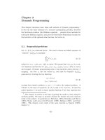
Figure 5.6.1: Graph of f(Σ) =
Σ(R+Q)+QR
Σ+R
, Q = R =1,
against the 45-degree line. Iterations on the Riccati equation
for Σ
t
converge to the fixed point.
For this problem, A =1,CC

= Q, G = 1, causing the Kalman filtering
equations to become
K
t

=
Σ
t
Σ
t
+ R
(5.6.8a)
Σ
t+1
=Σ
t
+ Q −
Σ
2
t
Σ
t
+ R
. (5.6.8b)
The second equation can be rewritten
Σ
t+1
=
Σ
t
(R + Q)+QR
Σ
t
+ R
. (5.6.9)

For Q = R = 1 , Figure 4.1 plots the function f(Σ) =
Σ(R+Q)+QR
Σ+R
appearing on
the right side of equation (5.6.9) for values Σ ≥ 0 against the 45-degree line.
124 Linear Quadratic Dynamic Programming
Note that f(0) = Q. This graph identifies the fixed point of iterations on f (Σ)
as the intersection of f(·) and the 45-degree line. That the slope of f(·)isless
than unity at the intersection assures us that the iterations on f will converge
as t → +∞ starting from any Σ
0
≥ 0.
Muth studied the solution of this problem as t →∞.Evidently,Σ
t
→
Σ
∞
≡ Σ is the fixed point of a graph like Figure 4.1. Then K
t
→ K and the
formula for ˆx
t+1
becomes
ˆx
t+1
=(1−K)ˆx
t
+ Ky
t
(5.6.10)

where K =
Σ
Σ+R
∈ (0, 1). This is a version of Cagan’s adaptive expectations
formula. Iterating backward on equation (5.6.10) gives ˆx
t+1
= K

t
j=0
(1 −
K)
j
y
t−j
+K(1−K)
t+1
ˆx
0
, which is a version of Cagan and Friedman’s geometric
distributed lag formula. Using equations (5.6.7), we find that E[y
t+j
|y
t
]=
E[x
t+j
|y
t
]=ˆx

t+1
for all j ≥ 1. This result in conjunction with equation
(5.6.10) establishes that the adaptive expectation formula (5.6.10) gives the
optimal forecast of y
t+j
for all horizons j ≥ 1. This finding itself is remarkable
and special because for most processes the optimal forecast will depend on the
horizon. That there is a single optimal forecast for all horizons in one sense
justifies the term “permanent income” that Milton Friedman (1955) chose to
describe the forecast.
The dependence of the forecast on horizon can be studied using the formulas
E

x
t+j
|y
t−1

= A
j
ˆx
t
(5.6.11a)
E

y
t+j
|y
t−1


= GA
j
ˆx
t
(5.6.11b)
In the case of Muth’s example,
E

y
t+j
|y
t−1

=ˆy
t
=ˆx
t
∀j ≥ 0.
The Kalman filter 125
5.6.2. Jovanovic’s example
In chapter 6, we will describe a version of Jovanovic’s (1979) matching model,
at the core of which is a “signal-extraction” problem that simplifies Muth’s
problem. Let x
t
,y
t
be scalars with A =1,C =0,G =1,R > 0. Let x
0
be Gaussian with mean µ and variance Σ
0

. Interpret x
t
(which is evidently
constant with this specification) as the hidden value of θ , a “match parameter.”
Let y
t
denote the history of y
s
from s =0tos = t. Define m
t
≡ ˆx
t+1
≡ E[θ|y
t
]
and Σ
t+1
= E(θ −m
t
)
2
. Then in this particular case the Kalman filter becomes
m
t
=(1−K
t
) m
t−1
+ K
t

y
t
(5.6.12a)
K
t
=
Σ
t
Σ
t
+ R
(5.6.12b)
Σ
t+1
=
Σ
t
R
Σ
t
+ R
. (5.6.12c)
The recursions are to be initiated from (m
−1
, Σ
0
), a pair that embodies all
“prior” knowledge about the position of the system. It is easy to see from
Figure 4.1 that when Q = 0, Σ = 0 is the limit point of iterations on equation
(5.6.12c) starting from any Σ

0
≥ 0. Thus, the value of the match parameter is
eventually learned.
It is instructive to write equation (5.6.12c)as
1
Σ
t+1
=
1
Σ
t
+
1
R
. (5.6.13)
The reciprocal of the variance is often called the precision of the estimate. Ac-
cording to equation (5.6.13) the precision increases without bound as t grows,
and Σ
t+1
→ 0.
16
We can represent the Kalman filter in the form (5.6.4) as
m
t+1
= m
t
+ K
t+1
a
t+1

which implies that
E (m
t+1
− m
t
)
2
= K
2
t+1
σ
2
a,t+1
16
As a further special case, consider when there is zero precision initially
(Σ
0
=+∞). Then solving the difference equation (5.6.13) gives
1
Σ
t
= t/R.
Substituting this into equations (5.6.12) gives K
t
=(t +1)
−1
, so that the
Kalman filter becomes m
0
= y

0
and m
t
=[1−(t +1)
−1
]m
t−1
+(t +1)
−1
y
t
,
which implies that m
t
=(t +1)
−1

t
s=0
y
t
, the sample mean, and Σ
t
= R/t.
126 Linear Quadratic Dynamic Programming
where a
t+1
= y
t+1
−m

t
and the variance of a
t
is equal to σ
2
a,t+1
=(Σ
t+1
+ R)
from equation (5.6.5). This implies
E (m
t+1
− m
t
)
2
=
Σ
2
t+1
Σ
t+1
+ R
.
For the purposes of our discrete time counterpart of the Jovanovic model in
chapter 6, it will be convenient to represent the motion of m
t+1
by means of
the equation
m

t+1
= m
t
+ g
t+1
u
t+1
where g
t+1
≡

Σ
2
t+1
Σ
t+1
+R

.5
and u
t+1
is a standardized i.i.d. normalized and
standardized with mean zero and variance 1 constructed to obey g
t+1
u
t+1
≡
K
t+1
a

t+1
.
5.7. Concluding remarks
In exchange for their restrictions, the linear quadratic dynamic optimization
models of this chapter acquire tractability. The Bellman equation leads to Ric-
cati difference equations that are so easy to solve numerically that the curse of
dimensionality loses most of its force. It is easy to solve linear quadratic control
or filtering with many state variables. That it is difficult to solve those prob-
lems otherwise is why linear quadratic approximations are used so widely. We
describe those approximations in appendix B to this chapter.
In chapter 7, we go beyond the single-agent optimization problems of this
chapter and the previous one to study systems with multiple agents simultane-
ously solving such problems. We introduce two equilibrium concepts for restrict-
ing how different agents’ decisions are reconciled. To facilitate the analysis, we
describe and illustrate those equilibrium concepts in contexts where each agent
solves an optimal linear regulator problem.
Linear-quadratic approximations 127
A. Matrix formulas
Let (z,x, a)eachben × 1 vectors, A, C, D,andV each be (n ×n) matrices,
B an (n ×m) matrix, and y an (m ×1) vector. Then
∂a

x
∂x
= a,
∂x

Ax
∂x
=(A +

A

)x,
∂
2
(x

Ax)
∂x∂x

=(A + A

),
∂x

Ax
∂A
= xx

,
∂y

Bz
∂y
= Bz,
∂y

Bz
∂z
= B


y,
∂y

Bz
∂B
= yz

.
The equation
A

VA+ C = V
to be solved for V , is called a discrete Lyapunov equation; and its generalization
A

VD+ C = V
is called the discrete Sylvester equation. The discrete Sylvester equation has a
unique solution if and only if the eigenvalues {λ
i
} of A and {δ
j
} of D satisfy
the condition λ
i
δ
j
=1∀ i, j.
B. Linear-quadratic approximations
This appendix describes an important use of the optimal linear regulator: to

approximate the solution of more complicated dynamic programs.
17
Optimal
linear regulator problems are often used to approximate problems of the fol-
lowing form: maximize over {u
t
}
∞
t=0
E
0
∞

t=0
β
t
r (z
t
)(5.B.1)
x
t+1
= Ax
t
+ Bu
t
+ Cw
t+1
(5.B.2)
where {w
t+1

} is a vector of i.i.d. random disturbances with mean zero and finite
variance, and r(z
t
) is a concave and twice continuously differentiable function
of z
t
≡

x
t
u
t

. All nonlinearities in the original problem are absorbed into the
composite function r(z
t
).
17
Kydland and Prescott (1982) used such a method, and so do many of their
followers in the real business cycle literature. See King, Plosser, and Rebelo
(1988) for related methods of real business cycle models.
128 Linear Quadratic Dynamic Programming
5.B.1. An example: the stochastic growth model
Take a parametric version of Brock and Mirman’s stochastic growth model,
whose social planner chooses a policy for {c
t
,a
t+1
}
∞

t=0
to maximize
E
0
∞

t=0
β
t
ln c
t
where
c
t
+ i
t
= Aa
α
t
θ
t
a
t+1
=(1−δ) a
t
+ i
t
ln θ
t+1
= ρ ln θ

t
+ w
t+1
where {w
t+1
} is an i.i.d. stochastic process with mean zero and finite variance,
θ
t
is a technology shock, and
˜
θ
t
≡ ln θ
t
. To get this problem into the form
(5.B.1)–(5.B.2), take x
t
=

a
t
˜
θ
t

, u
t
= i
t
,andr(z

t
)=ln(Aa
α
t
exp
˜
θ
t
− i
t
),
and we write the laws of motion as


1
a
t+1
˜
θ
t+1


=


100
0(1−δ)0
00ρ





1
a
t
˜
θ
t


+


0
1
0


i
t
+


0
0
1


w
t+1

where it is convenient to add the constant 1 as the first component of the state
vector.
5.B.2. Kydland and Prescott’s method
We want to replace r(z
t
)byaquadraticz

t
Mz
t
.Wechooseapoint¯z and
approximate with the first two terms of a Taylor series:
18
ˆr (z)=r (¯z)+(z − ¯z)

∂r
∂z
+
1
2
(z − ¯z)

∂
2
r
∂z∂z

(z − ¯z) .
(5.B.3)
If the state x

t
is n × 1 and the control u
t
is k × 1, then the vector z
t
is
(n + k) × 1. Let e be the (n + k) × 1 vector with 0’s everywhere except for
18
This setup is taken from McGrattan (1994) and Anderson, Hansen, Mc-
Grattan, and Sargent (1996).
Linear-quadratic approximations 129
a 1 in the row corresponding to the location of the constant unity in the state
vector, so that 1 ≡ e

z
t
for all t.
Repeatedly using z

e = e

z = 1, we can express equation (5.B.3) as
ˆr (z)=z

Mz,
where
M =e

r (¯z) −


∂r
∂z


¯z +
1
2
¯z

∂
2
r
∂z∂z

¯z

e

+
1
2

∂r
∂z
e

− e¯z

∂
2

r
∂z∂z

−
∂
2
r
∂z∂z

¯ze

+ e
∂r
∂z


+
1
2

∂
2
r
∂z∂z


where the partial derivatives are evaluated at ¯z . Partition M ,sothat
z

Mz ≡


x
u



M
11
M
12
M
21
M
22

x
u

=

x
u



RW
W

Q


x
u

.
5.B.3. Determination of ¯z
Usually, the point ¯z is chosen as the (optimal) stationary state of the non-
stochastic version of the original nonlinear model:
∞

t=0
β
t
r (z
t
)
x
t+1
= Ax
t
+ Bu
t
.
This stationary point is obtained in these steps:
1. Find the Euler equations.
2. Substitute z
t+1
= z
t
≡ ¯z into the Euler equations and transition laws,
and solve the resulting system of nonlinear equations for ¯z. This pur-

pose can be accomplished, for example, by using the nonlinear equation
solver fsolve.m in Matlab.
130 Linear Quadratic Dynamic Programming
5.B.4. Log linear approximation
For some problems Christiano (1990) has advocated a quadratic approximation
in logarithms. We illustrate his idea with the stochastic growth example. Define
˜a
t
=loga
t
,
˜
θ
t
=logθ
t
.
Christiano’s strategy is to take ˜a
t
,
˜
θ
t
as the components of the state and write
the law of motion as


1
˜a
t+1

˜
θ
t+1


=


100
000
00ρ




1
˜a
t
˜
θ
t


+


0
1
0



u
t
+


0
0
1


w
t+1
where the control u
t
is ˜a
t+1
.
Express consumption as
c
t
= A (exp ˜a
t
)
α

exp
˜
θ
t


+(1− δ)exp˜a
t
− exp ˜a
t+1
.
Substitute this expression into ln c
t
≡ r(z
t
), and proceed as before to obtain
the second-order Taylor series approximation about ¯z .
5.B.5. Trend removal
It is conventional in the real business cycle literature to specify the law of motion
for the technology shock θ
t
by
˜
θ
t
=log

θ
t
γ
t

,γ>1
˜
θ

t+1
= ρ
˜
θ
t
+ w
t+1
, |ρ| < 1. (5.B.4)
This inspires us to write the law of motion for capital as
γ
a
t+1
γ
t+1
=(1−δ)
a
t
γ
t
+
i
t
γ
t
Exercises 131
or
γ exp ˜a
t+1
=(1−δ)exp˜a
t

+exp

˜
i
t

(5.B.5)
where ˜a
t
≡ log

a
t
γ
t

,
˜
i
t
=log

i
t
γ
t

. By studying the Euler equations for a model
with a growing technology shock (γ>1), we can show that there exists a
steady state for ˜a

t
, but not for a
t
. Researchers often construct linear-quadratic
approximations around the nonstochastic steady state of ˜a.
Exercises
Exercise 5.1 Consider the modified version of the optimal linear regulator
problem where the objective is to maximize
−
∞

t=0
β
t
{x

t
Rx
t
+ u

t
Qu
t
+2u

t
Hx
t
}

subject to the law of motion:
x
t+1
= Ax
t
+ Bu
t
.
Here x
t
is an n × 1 state vector, u
t
is a k × 1 vector of controls, and x
0
is a
given initial condition. The matrices R, Q are positive definite and symmetric.
The maximization is with respect to sequences {u
t
,x
t
}
∞
t=0
.
a. Show that the optimal policy has the form
u
t
= −(Q + βB

PB)

−1
(βB

PA+ H) x
t
,
where P solves the algebraic matrix Riccati equation
P = R + βA

PA− (βA

PB + H

)(Q + βB

PB)
−1
(βB

PA+ H) . (5.6)
b. Write a Matlab program to solve equation (5.6) by iterating on P starting
from P being a matrix of zeros.
Exercise 5.2 Verify that equations (5.2.10) and (5.2.11) implement the policy
improvement algorithm for the discounted linear regulator problem.