Recursive macroeconomic theory, Thomas Sargent 2nd Ed - Chapter 8 pptx

Chapter 8
Equilibrium with Complete Markets
8.1. Time-0 versus sequential trading
This chapter describes competitive equilibria for a pure exchange infinite horizon
economy with stochastic endowments. This economy is useful for studying risk
sharing, asset pricing, and consumption. We describe two market structures:
an Arrow-Debreu structure with complete markets in dated contingent claims
all traded at time 0, and a sequential-trading structure with complete one-
period Arrow securities. These two entail different assets and timings of trades,
but have identical consumption allocations. Both are referred to as complete
market economies. They allow more comprehensive sharing of risks than do
the incomplete markets economies to be studied in chapters 16 and 17, or the
economies with imperfect enforcement or imperfect information in chapters 19
and 20.
8.2. The physical setting: preferences and endowments
In each period t ≥ 0, there is a realization of a stochastic event s
t
∈ S .Let
the history of events up and until time t be denoted s
t
=[s
0
,s
1
, ,s
t
]. The
unconditional probability of observing a particular sequence of events s
t
is given
by a probability measure π

t
(s
t
). We write conditional probabilities as π
t
(s
t
|s
τ
)
which is the probability of observing s
t
conditional upon the realization of s
τ
.
In this chapter, we shall assume that trading occurs after observing s
0
,which
is here captured by setting π
0
(s
0
) = 1 for the initially given value of s
0
.
1
In section 8.9 we shall follow much of the literatures in macroeconomics
and econometrics and assume that π
t
(s

t
) is induced by a Markov process. We
1
Most of our formulas carry over to the case where trading occurs before s
0
has been realized; just postulate a nondegenerate probability distribution π
0
(s
0
)
over the initial state.
– 203 –
204 Equilibrium with Complete Markets
wait to impose that special assumption because some important findings do not
require making that assumption.
There are I agents named i =1, ,I.Agenti owns a stochastic en-
dowment of one good y
i
t
(s
t
) that depends on the history s
t
. The history s
t
is
publicly observable. Household i purchases a history-dependent consumption
plan c
i
= {c

i
t
(s
t
)}
∞
t=0
and orders these consumption streams by
U

c
i

=
∞

t=0

s
t
β
t
u

c
i
t

s
t


π
t

s
t

. (8.2.1)
The right side is equal to E
0

∞
t=0
β
t
u(c
i
t
), where E
0
is the mathematical ex-
pectation operator, conditioned on s
0
.Hereu(c) is an increasing, twice con-
tinuously differentiable, strictly concave function of consumption c ≥ 0ofone
good. The utility function satisfies the Inada condition
2
lim
c↓0
u


(c)=+∞.
A feasible allocation satisfies

i
c
i
t

s
t

≤

i
y
i
t

s
t

(8.2.2)
for all t and for all s
t
.
2
The chief role of this Inada condition in this chapter will be to guarantee
interior solutions, i.e., the consumption of each agent is strictly positive in every
period.

Alternative trading arrangements 205
8.3. Alternative trading arrangements
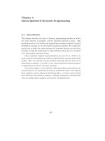
For a two-event stochastic process s
t
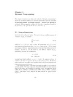
∈ S = {0, 1}, the trees in Figures 8.3.1
and 8.3.2. give two portraits of how the history of the economy unfolds. From
the perspective of time 0 given s
0
= 0, Figure 8.3.1 portrays the full variety
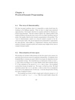
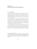
of prospective histories that are possible up to time 3. Figure 8.3.2 portrays a
particular history that it is known the economy has indeed followed up to time
2, together with the two possible one-period continuations into period 3 that
can occur after that history.
(0,1,1,1)
(0,1,1,0)
(0,1,0,1)
(0,1,0,0)
(0,0,1,1)
(0,0,1,0)
(0,0,0,1)
(0,0,0,0)
t=0 t=1 t=2 t=3
Figure 8.3.1: The Arrow-Debreu commodity space for a
two-state Markov chain. At time 0, there are trades in time
t = 3 goods for each of the eight ‘nodes’ or ‘histories’ that
can possibly be reached starting from the node at time 0.
In this chapter we shall study two distinct trading arrangements that corre-
spond, respectively, to the two views of the economy in Figures 8.3.1 and 8.3.2.
OneiswhatweshallcalltheArrow-Debreu structure. Here markets meet at
time 0 to trade claims to consumption at all times t>0 and that are contingent

on all possible histories up to t, s
t
. In that economy, at time 0, households
206 Equilibrium with Complete Markets
trade claims on the time t consumption good at all nodes s
t
.Aftertime0,
no further trades occur. The other economy has sequential trading of only one-
period ahead state contingent claims. Here trades occur at each date t ≥ 0.
Trades for history s
t+1
–contingent date t + 1 goods occur only at the particular
date t history s
t
that has been reached at t, as in Fig. 8.3.2. Remarkably,
these two trading arrangements will support identical equilibrium allocations.
Those allocations share the notable property of being functions only of the ag-
gregate endowment realization. They do depend neither on the specific history
preceding the outcome for the aggregate endowment nor on the realization of
individual endowments.
8.3.1. History dependence
In principle the situation of household i at time t might very well depend on the
history s
t
. A natural measure of household i’s luck in life is {y
i
0
(s
0
),y

i
1
(s
1
), ,
y
i
t
(s
t
)}. This obviously depends on the history s
t
. A question that will occupy
us in this chapter and in chapter 19 is whether after trading, the household’s
consumption allocation at time t is history dependent or whether it depends
only on the current aggregate endowment. Remarkably, in the complete markets
models of this chapter, the consumption allocation at time t will depend only
on the aggregate endowment realization. The market incompleteness of chapter
17 and the information and enforcement frictions of chapter 19 will break that
result and put history dependence into equilibrium allocations.
t=1t=0 t=2 t=3
(1|0,0,1)
(0|0,0,1)
Figure 8.3.2: The commodity space with Arrow securities.
At date t = 2, there are trades in time 3 goods for only those
time t = 3 nodes that can be reached from the realized time
t =2 history (0, 0, 1).
Pareto problem 207
8.4. Pareto problem
As a benchmark against which to measure allocations attained by a market

economy, we seek efficient allocations. An allocation is said to be efficient if
it is Pareto optimal: it has the property that any reallocation that makes one
household strictly better off also makes one or more other households worse off.
We can find efficient allocations by posing a Pareto problem for a fictitious social
planner. The planner attaches nonnegative Pareto weights λ
i
,i =1, ,I on
the consumers and chooses allocations c
i
,i=1, ,I to maximize
W =
I

i=1
λ
i
U

c
i

(8.4.1)
subject to (8.2.2). We call an allocation efficient if it solves this problem for
some set of nonnegative λ
i
’s. Let θ
t
(s
t
) be a nonnegative Lagrange multiplier

on the feasibility constraint (8.2.2) for time t and history s
t
,andformthe
Lagrangian
L =
∞

t=0

s
t

I

i=1
λ
i
β
t
u

c
i
t

s
t

π
t


s
t

+ θ
t

s
t

I

i=1

y
i
t

s
t

− c
i
t

s
t


The first-order condition for maximizing L with respect to c

i
t
(s
t
)is
β
t
u


c
i
t

s
t

π
t

s
t

= λ
−1
i
θ
t

s

t

(8.4.2)
for all i, t, s
t
.Takingtheratioof(8.4.2) for consumers i and 1 gives
u


c
i
t
(s
t
)

u

(c
1
t
(s
t
))
=
λ
1
λ
i
which implies

c
i
t

s
t

= u
−1

λ
−1
i
λ
1
u


c
1
t

s
t

. (8.4.3)
Substituting (8.4.3) into feasibility condition (8.2.2) at equality gives

i
u

−1

λ
−1
i
λ
1
u


c
1
t

s
t

=

i
y
i
t

s
t

. (8.4.4)
Equation (8.4.4) is one equation in c
1

t
(s
t
). The right side of (8.4.4) is the
realized aggregate endowment, so the left side is a function only of the aggre-
gate endowment. Thus, c
1
t
(s
t
) depends only on the current realization of the
208 Equilibrium with Complete Markets
aggregate endowment and neither on the specific history s
t
leading up to that
outcome nor on the realization of individual endowments. Equation (8.4.3)
then implies that for all i, c
i
t
(s
t
) depends only on the aggregate endowment
realization. We thus have:
Proposition 1: An efficient allocation is a function of the realized aggre-
gate endowment and depends neither on the specific history leading up to that
outcome nor on the realizations of individual endowments; c
i
t
(s
t

)=c
i
τ
(˜s
τ
)for
s
t
and ˜s
τ
such that

j
y
j
t
(s
t
)=

j
y
j
τ
(˜s
τ
).
To compute the optimal allocation, first solve (8.4.4) for c
1
t

(s
t
), then solve
(8.4.3) for c
i
t
(s
t
). Note from (8.4.3) that only the ratios of the Pareto weights
matter, so that we are free to normalize the weights, e.g., to impose

i
λ
i
=1.
8.4.1. Time invariance of Pareto weights
Through equations (8.4.3) and (8.4.4), the allocation c
i
t
(s
t
) assigned to con-
sumer i depends in a time-invariant way on the aggregate endowment

j
y
j
t
(s
t

).
Consumer i’s share of the aggregate varies directly with his Pareto weight λ
i
.
In chapter 19, we shall see that the constancy through time of the Pareto weights
{λ
j
}
I
j=1
is a tell tale sign that there are no enforcement or information-related
incentive problems in this economy. When we inject those problems into our
environment in chapter 19, the time-invariance of the Pareto weights evaporates.
8.5. Time-0 trading: Arrow-Debreu securities
We now describe how an optimal allocation can be attained by a competitive
equilibrium with the Arrow-Debreu timing. Households trade dated history-
contingent claims to consumption. There is a complete set of securities. Trades
occur at time 0, after s
0
has been realized. At t = 0, households can exchange
claims on time-t consumption, contingent on history s
t
at price q
0
t
(s
t
). The
superscript 0 refers to the date at which trades occur, while the subscript t refers
to the date that deliveries are to be made. The household’s budget constraint

Time-0 trading: Arrow-Debreu securities 209
is
∞

t=0

s
t
q
0
t

s
t

c
i
t

s
t

≤
∞

t=0

s
t
q

0
t

s
t

y
i
t

s
t

. (8.5.1)
The household’s problem is to choose c
i
to maximize expression (8.2.1) subject
to inequality (8.5.1). Here q
0
t
(s
t
) is the price of time t consumption contingent
on history s
t
at t in terms of an abstract unit of account or numeraire.
Underlying the single budget constraint (8.5.1) is the fact that multilateral
trades are possible through a clearing operation that keeps track of net claims.
3
All trades occur at time 0. After time 0, trades that were agreed to at time 0

are executed, but no more trades occur.
Each household has a single budget constraint (8.5.1) to which we attach a
Lagrange multiplier µ
i
. We obtain the first-order conditions for the household’s
problem:
∂U

c
i

∂c
i
t
(s
t
)
= µ
i
q
0
t

s
t

. (8.5.2)
The left side is the derivative of total utility with respect to the time-t,history-s
t
component of consumption. Each household has its own µ

i
that is independent
of time. Note also that with specification (8.2.1) of the utility functional, we
have
∂U

c
i

∂c
i
t
(s
t
)
= β
t
u


c
i
t

s
t

π
t


s
t

. (8.5.3)
This expression implies that equation (8.5.2) can be written
β
t
u


c
i
t

s
t

π
t

s
t

= µ
i
q
0
t

s

t

. (8.5.4)
We use the following definitions:
Definitions: A price system is a sequence of functions {q
0
t
(s
t
)}
∞
t=0
.An
allocation is a list of sequences of functions c
i
= {c
i
t
(s
t
)}
∞
t=0
,oneforeachi.
Definition: A competitive equilibrium is a feasible allocation and a price
system such that, given the price system, the allocation solves each household’s
problem.
3
In the language of modern payments systems, this is a system with net
settlements, not gross settlements, of trades.

210 Equilibrium with Complete Markets
Notice that equation (8.5.4) implies
u


c
i
t
(s
t
)

u


c
j
t
(s
t
)

=
µ
i
µ
j
(8.5.5)
for all pairs (i, j). Thus, ratios of marginal utilities between pairs of agents are
constant across all histories and dates.

An equilibrium allocation solves equations (8.2.2), (8.5.1), and (8.5.5).
Note that equation (8.5.5) implies that
c
i
t

s
t

= u
−1

u


c
1
t

s
t

µ
i
µ
1

. (8.5.6)
Substituting this into equation (8.2.2) at equality gives


i
u
−1

u


c
1
t

s
t

µ
i
µ
1

=

i
y
i
t

s
t

. (8.5.7)

The right side of equation (8.5.7) is the current realization of the aggregate
endowment. It does not per se depend on the specific history leading up this
outcome; therefore, the left side, and so c
1
t
(s
t
), must also depend only on the
current aggregate endowment. It follows from equation (8.5.6 ) that the equi-
librium allocation c
i
t
(s
t
)foreachi depends only on the economy’s aggregate
endowment. We summarize this analysis in the following proposition:
Proposition 2: The competitive equilibrium allocation is a function of
the realized aggregate endowment and depends neither on the specific history
leading up to that outcome nor on the realizations of individual endowments;
c
i
t
(s
t
)=c
i
τ
(˜s
τ
)fors

t
and ˜s
τ
such that

j
y
j
t
(s
t
)=

j
y
j
τ
(˜s
τ
).
Time-0 trading: Arrow-Debreu securities 211
8.5.1. Equilibrium pricing function
Suppose that c
i
, i =1, ,I is an equilibrium allocation. Then the marginal
condition (8.5.2) or (8.5.4) gives the price system q
0
t
(s
t

) as a function of the
allocation to household i, for any i. Note that the price system is a stochastic
process. Because the units of the price system are arbitrary, one of the prices
can be normalized at any positive value. We shall set q
0
0
(s
0
) = 1, putting the
price system in units of time-0 goods. This choice implies that µ
i
= u

[c
i
0
(s
0
)]
for all i.
8.5.2. Optimality of equilibrium allocation
A competitive equilibrium allocation is a particular Pareto optimal allocation,
one that sets the Pareto weights λ
i
= µ
−1
i
,whereµ
i
,i=1, ,I is the unique

(up to multiplication by a positive scalar) set of Pareto weights associated with
the competitive equilibrium. Furthermore, at the competitive equilibrium allo-
cation, the shadow prices θ
t
(s
t
) for the associated planning problem equal the
prices q
0
t
(s
t
) for goods to be delivered at date t contingent on history s
t
as-
sociated with the Arrow-Debreu competitive equilibrium. That the allocations
for the planning problem and the competitive equilibrium are aligned reflects
the two fundamental theorems of welfare economics (see Mas-Colell, Whinston,
Green (1995)).
8.5.3. Equilibrium computation
To compute an equilibrium, we have somehow to determine ratios of the La-
grange multipliers, µ
i
/µ
1
, i =1, ,I, that appear in equations (8.5.6), (8.5.7).
The following Negishi algorithm accomplishes this.
4
1. Fix a positive value for one µ
i

,sayµ
1
throughout the algorithm. Guess
some positive values for the remaining µ
i
’s. Then solve equations (8.5.6),
(8.5.7) for a candidate consumption allocation c
i
,i=1, ,I.
2. Use (8.5.4) for any household i to solve for the price system q
0
t
(s
t
).
4
See Negishi (1960).
212 Equilibrium with Complete Markets
3. For i =1, ,I, check the budget constraint (8.5.1). For those i’s for
which the cost of consumption exceeds the value of their endowment, raise
µ
i
, while for those i’s for which the reverse inequality holds, lower µ
i
.
4. Iterate to convergence on steps 1 – 3.
Multiplying all of the µ
i
’s by a positive scalar amounts simply to a change
in units of the price system. That is why we are free to normalize as we have in

step 1.
8.5.4. Interpretation of trading arrangement
In the competitive equilibrium, all trades occur at t = 0 in one market. Deliv-
eries occur after t = 0, but no more trades. A vast clearing or credit system
operates at t = 0. It assures that condition (8.5.1) holds for each household
i. A symptom of the once-and-for-all trading arrangement is that each house-
hold faces one budget constraint that accounts for all trades across dates and
histories.
In section 8.8, we describe another trading arrangement with more trading
dates but fewer securities at each date.
8.6. Examples
8.6.1. Example 1: Risk sharing
Suppose that the one-period utility function is of the constant relative risk-
aversion form
u (c)=(1−γ)
−1
c
1−γ
,γ>0.
Then equation (8.5.5) implies

c
i
t

s
t

−γ
=


c
j
t

s
t


−γ
µ
i
µ
j
or
c
i
t

s
t

= c
j
t

s
t



µ
i
µ
j

−
1
γ
. (8.6.1)
Examples 213
Equation (8.6.1) states that time-t elements of consumption allocations to dis-
tinct agents are constant fractions of one another. With a power utility function,
it says that individual consumption is perfectly correlated with the aggregate
endowment or aggregate consumption.
5
The fractions of the aggregate endowment assigned to each individual are
independent of the realization of s
t
. Thus, there is extensive cross-history
and cross-time consumption smoothing. The constant-fractions-of-consumption
characterization comes from these two aspects of the theory: (1) complete mar-
kets, and (2) a homothetic one-period utility function.
8.6.2. Example 2: No aggregate uncertainty
Let the stochastic event s
t
take values on the unit interval [0, 1]. There are
two households, with y
1
t
(s

t
)=s
t
and y
2
t
(s
t
)=1− s
t
. Note that the aggregate
endowment is constant,

i
y
i
t
(s
t
) = 1. Then equation (8.5.7) implies that
c
1
t
(s
t
) is constant over time and across histories, and equation (8.5.6 ) implies
that c
2
t
(s

t
) is also constant. Thus the equilibrium allocation satisfies c
i
t
(s
t
)=¯c
i
for all t and s
t
,fori =1, 2. Then from equation (8.5.4),
q
0
t

s
t

= β
t
π
t

s
t

u


¯c

i

µ
i
, (8.6.2)
for all t and s
t
,fori =1, 2. Household i’s budget constraint implies
u


¯c
i

µ
i
∞

t=0

s
t
β
t
π
t

s
t


¯c
i
− y
i
t

s
t

=0.
Solving this equation for ¯c
i
gives
¯c
i
=(1−β)
∞

t=0

s
t
β
t
π
t

s
t


y
i
t

s
t

. (8.6.3)
5
Equation (8.6.1) implies that conditional on the history s
t
,timet con-
sumption c
i
t
(s
t
) is independent of the household’s individual endowment y
i
t
(s
t
).
Mace (1991), Cochrane (1991), and Townsend (1994) have all tested and rejected
versions of this conditional independence hypothesis. In chapter 19, we study
how particular impediments to trade can help explain these rejections.
214 Equilibrium with Complete Markets
Summing equation (8.6.3) verifies that ¯c
1
+¯c

2
=1.
6
8.6.3. Example 3: Periodic endowment processes
Consider the special case of the previous example in which s
t
is deterministic
and alternates between the values 1 and 0; s
0
=1,s
t
=0fort odd, and s
t
=1
for t even. Thus, the endowment processes are perfectly predictable sequences
(1, 0, 1, ) for the first agent and (0, 1, 0, ) for the second agent. Let ˜s
t
be
the history of (1, 0, 1, )uptot.Evidently,π
t
(˜s
t
) = 1 , and the probability
assigned to all other histories up to t is zero. The equilibrium price system is
then
q
0
t

s

t

=

β
t
, if s
t
=˜s
t
;
0, otherwise ;
when using the time-0 good as numeraire, q
0
0
(˜s
0
) = 1. From equation (8.6.3),
we have
¯c
1
=(1−β)
∞

j=0
β
2j
=
1
1+β

, (8.6.4a)
¯c
2
=(1−β) β
∞

j=0
β
2j
=
β
1+β
. (8.6.4b)
Consumer 1 consumes more every period because he is richer by virtue of re-
ceiving his endowment earlier.
6
If we let β
−1
=1+r,wherer is interpreted as the risk-free rate of interest,
then note that (8.6.3)canbeexpressedas
¯c
i
=

r
1+r

E
0
∞


t=0
(1 + r)
−t
y
i
t

s
t

.
Hence, equation (8.6.3) is a version of Friedman’s permanent income model,
which asserts that a household with zero financial assets consumes the annu-
ity value of its ‘human wealth’ defined as the expected discounted value of its
labor income (which for present purposes we take to be y
i
t
(s
t
)). Of course, in
the present example, the household completely smooths its consumption across
time and histories, something that the household in Friedman’s model typically
cannot do. See chapter 16.
Primer on asset pricing 215
8.7. Primer on asset pricing
Many asset-pricing models assume complete markets and price an asset by
breaking it into a sequence of history-contingent claims, evaluating each com-
ponent of that sequence with the relevant “state price deflator” q
0

t
(s
t
), then
adding up those values. The asset is viewed as redundant , in the sense that it
offers a bundle of history-contingent dated claims, each component of which has
already been priced by the market. While we shall devote chapter 13 entirely
to asset-pricing theories, it is useful to give some pricing formulas at this point
because they help illustrate the complete market competitive structure.
8.7.1. Pricing redundant assets
Let {d
t
(s
t
)}
∞
t=0
be a stream of claims on time t,historys
t
consumption, where
d
t
(s
t
) is a measurable function of s
t
. The price of an asset entitling the owner
to this stream must be
p
0

0
(s
0
)=
∞

t=0

s
t
q
0
t

s
t

d
t

s
t

. (8.7.1)
If this equation did not hold, someone could make unbounded profits by syn-
thesizing this asset through purchases or sales of history-contingent dated com-
modities and then either buying or selling the asset. We shall elaborate this
arbitrage argument below and later in chapter 13 on asset pricing.
8.7.2. Riskless consol
As an example, consider the price of a riskless consol, that is, an asset offering

to pay one unit of consumption for sure each period. Then d
t
(s
t
) = 1 for all t
and s
t
, and the price of this asset is
∞

t=0

s
t
q
0
t

s
t

. (8.7.2)
216 Equilibrium with Complete Markets
8.7.3. Riskless strips
As another example, consider a sequence of strips of payoffs on the riskless
consol. The time-t strip is just the payoff process d
τ
=1ifτ = t ≥ 0, and
0 otherwise. Thus, the owner of the strip is entitled only to the time-t coupon.
The value of the time-t strip at time 0 is evidently


s
t
q
0
t

s
t

.
Compare this to the price of the consol (8.7.2). Of course, we can think of the
t-period riskless strip as simply a t-period zero-coupon bond. See section 2.7
for an account of a closely related model of yields on such bonds.
8.7.4. Tail assets
Return to the stream of dividends {d
t
(s
t
)}
t≥0
generated by the asset priced in
equation (8.7.1). For τ ≥ 1, suppose that we strip off the first τ − 1peri-
ods of the dividend and want to get the time-0 value of the dividend stream
{d
t
(s
t
)}
t≥τ

. Specifically, we seek this asset value for each possible realization
of s
τ
.Letp
0
τ
(s
τ
) be the time-0 price of an asset that entitles the owner to
dividend stream {d
t
(s
t
)}
t≥τ
if history s
τ
is realized,
p
0
τ
(s
τ
)=

t≥τ

s
t
|s

τ
q
0
t

s
t

d
t

s
t

, (8.7.3)
where the summation over s
t
|s
τ
means that we sum over all possible histories
˜s
t
such that ˜s
τ
= s
τ
. The units of the price are time-0 (state-s
0
) goods per
unit (the numeraire) so that q

0
0
(s
0
) = 1. To convert the price into units of time
τ ,historys
τ
consumption goods, divide by q
0
τ
(s
τ
)toget
p
τ
τ
(s
τ
) ≡
p
0
τ
(s
τ
)
q
0
τ
(s
τ

)
=

t≥τ

s
t
|s
τ
q
0
t
(s
t
)
q
0
τ
(s
τ
)
d
t

s
t

. (8.7.4)
Notice that
7

q
τ
t

s
t

≡
q
0
t
(s
t
)
q
0
τ
(s
τ
)
=
β
t
u


c
i
t
(s

t
)

π
t
(s
t
)
β
τ
u

[c
i
τ
(s
τ
)] π
τ
(s
τ
)
= β
t−τ
u


c
i
t

(s
t
)

u

[c
i
τ
(s
τ
)]
π
t

s
t
|s
τ

.
(8.7.5)
7
Because the marginal conditions hold for all consumers, this condition holds
for all i.
Primer on asset pricing 217
Here q
τ
t
(s

t
) is the price of one unit of consumption delivered at time t,historys
t
in terms of the date-τ ,history-s
τ
consumption good; π
t
(s
t
|s
τ
) is the probability
of history s
t
conditional on history s
τ
at date τ .Thus,thepriceatt for the
“tail asset” is
p
τ
τ
(s
τ
)=

t≥τ

s
t
|s

τ
q
τ
t

s
t

d
t

s
t

. (8.7.6)
When we want to create a time series of, say, equity prices, we use the “tail
asset” pricing formula. An equity purchased at time τ entitles the owner to the
dividends from time τ forward. Our formula (8.7.6) expresses the asset price
in terms of prices with time τ ,historys
τ
good as numeraire.
Notice how formula (8.7.5) takes the form of a pricing function for a com-
plete markets economy with date- and history-contingent commodities, whose
markets have been reopened at date τ ,historys
τ
, given the wealth levels im-
plied by the tails of each household’s endowment and consumption streams. We
leave it as an exercise to the reader to prove the following proposition.
Proposition 3: Starting from the distribution of time t wealth that is
implicit in a time 0 Arrow-Debreu equilibrium, if markets are ‘reopened’ at

date t after history s
t
, no trades will occur. That is, given the price system
(8.7.5), all households choose to continue the tails of their original consumption
plans.
8.7.5. Pricing one period returns
The one-period version of equation (8.7.5) is
q
τ
τ +1

s
τ +1

= β
u


c
i
τ +1

s
τ +1

u

[c
i
τ

(s
τ
)]
π
τ +1

s
τ +1
|s
τ

.
The right side is the one-period pricing kernel at time τ . If we want to find the
price at time τ in history s
τ
of a claim to a random payoff ω(s
τ +1
), we use
p
τ
τ
(s
τ
)=

s
τ+1
q
τ
τ +1


s
τ +1

ω (s
τ +1
)
or
p
τ
τ
(s
τ
)=E
τ

β
u

(c
τ +1
)
u

(c
τ
)
ω (s
τ +1
)


, (8.7.7)
218 Equilibrium with Complete Markets
where E
τ
is the conditional expectation operator. We have deleted the i su-
perscripts on consumption, with the understanding that equation (8.7.7) is true
for any consumer i; we have also suppressed the dependence of c
τ
on s
τ
,which
is implicit.
Let R
τ +1
≡ ω(s
τ +1
)/p
τ
τ
(s
τ
) be the one-period gross return on the asset.
Then for any asset, equation (8.7.7) implies
1=E
τ

β
u


(c
τ +1
)
u

(c
τ
)
R
τ +1

≡ E
τ
[m
τ +1
R
τ +1
] . (8.7.8)
The term m
τ +1
≡ βu

(c
τ +1
)/u

(c
τ
) functions as a stochastic discount factor.
Like R

τ +1
, it is a random variable measurable with respect to s
τ +1
,givens
τ
.
Equation (8.7.8) is a restriction on the conditional moments of returns and
m
t+1
. Applying the law of iterated expectations to equation (8.7.8) gives the
unconditional moments restriction
1=E

β
u

(c
τ +1
)
u

(c
τ
)
R
τ +1

≡ E [m
τ +1
R

τ +1
] . (8.7.9)
In the next section, we display another market structure in which the one-
period pricing kernel q
t
t+1
(s
t+1
) also plays a decisive role. This structure uses
the celebrated one-period “Arrow securities,” the sequential trading of which
perfectly substitutes for the comprehensive trading of long horizon claims at
time 0.
8.8. Sequential trading: Arrow securities
This section describes an alternative market structure that preserves both the
equilibrium allocation and the key one-period asset-pricing formula (8.7.7).
Sequential trading: Arrow securities 219
8.8.1. Arrow securities
We build on an insight of Arrow (1964) that one-period securities are enough
to implement complete markets, provided that new one-period markets are re-
opened for trading each period. Thus, at each date t ≥ 0, trades occur in a
set of claims to one-period-ahead state-contingent consumption. We describe a
competitive equilibrium of this sequential trading economy. With a full array of
these one-period-ahead claims, the sequential trading arrangement attains the
same allocation as the competitive equilibrium that we described earlier.
8.8.2. Insight: wealth as an endogenous state variable
A key step in finding a sequential trading arrangement is to identify a variable
to serve as the state in a value function for the household at date t. We find
this state by taking an equilibrium allocation and price system for the (Arrow-
Debreu) time 0 trading structure and applying a guess and verify method. We
begin by asking the following question. In the competitive equilibrium where

all trading takes place at time 0, excluding its endowment, what is the implied
wealth of household i at time t after history s
t
?Inperiodt, conditional on
history s
t
, we sum up the value of the household’s purchased claims to current
and future goods net of its outstanding liabilities. Since history s
t
is realized,
we discard all claims and liabilities contingent on another initial history. For
example, household i’s net claim to delivery of goods in a future period τ ≥ t,
contingent on history ˜s
τ
such that ˜s
t
= s
t
,isgivenby[c
i
τ
(˜s
τ
) −y
i
t
(˜s
τ
)]. Thus,
the household’s wealth, or the value of all its current and future net claims,

expressed in terms of the date t,historys
t
consumption good is
Υ
i
t

s
t

=
∞

τ =t

s
τ
|s
t
q
t
τ
(s
τ
)

c
i
τ
(s

τ
) −y
i
t
(s
τ
)

. (8.8.1)
Notice that feasibility constraint (8.2.2) at equality implies that
I

i=1
Υ
i
t

s
t

=0, ∀t, s
t
.
In moving from the Arrow-Debreu economy to one with sequential trading,
we can match up the time t,historys
t
wealth of the household in the sequential
220 Equilibrium with Complete Markets
economy with the ‘tail wealth’ Υ
i

t
(s
t
) from the Arrow-Debreu computed in
equation (8.8.1). But first we have to say something about debt limits, a feature
that was absent in the Arrow-Debreu economy because we imposed (8.5.1)
8.8.3. Debt limits
In moving to the sequential formulation, we shall need to impose some restric-
tions on asset trades to prevent Ponzi schemes. We impose the weakest possible
restrictions in this section. We’ll synthesize restrictions that work by starting
from the equilibrium allocation of Arrow-Debreu economy (with time-0 mar-
kets), and find some state-by-state debt limits that suffice to support sequential
trading. Often we’ll refer to these weakest possible debt limits as the ‘natural
debt limits’. These limits come from the common sense requirement that it
has to be feasible for the consumer to repay his state contingent debt in every
possible state. Given our assumption that c
i
t
(s
t
) must be nonnegative, that
feasibility requirement leads to the natural debt limits that we now describe.
Let q
t
τ
(s
τ
) be the Arrow-Debreu price, denominated in units of the date
t,historys
t

consumption good. Consider the value of the tail of agent i’s
endowment sequence at time t in history s
t
:
A
i
t

s
t

=
∞

τ =t

s
τ
|s
t
q
t
τ
(s
τ
) y
i
τ
(s
τ

) . (8.8.2)
We call A
i
t
(s
t
)thenatural debt limit at time t and history s
t
.Itisthevalue
of the maximal amount that agent i can repay starting from that period, as-
suming that his consumption is zero forever. From now on, we shall require
that household i at time t − 1 and history s
t−1
cannot promise to pay more
than A
i
t
(s
t
) conditional on the realization of s
t
tomorrow, because it will not
be feasible for them to repay more. Note that household i at time t − 1 faces
one such borrowing constraint for each possible realization of s
t
tomorrow.
Sequential trading: Arrow securities 221
8.8.4. Sequential trading
There is a sequence of markets in one-period-ahead state-contingent claims to
wealth or consumption. At each date t ≥ 0, households trade claims to date

t + 1 consumption, whose payment is contingent on the realization of s
t+1
.Let
˜a
i
t
(s
t
) denote the claims to time t consumption, other than its endowment, that
household i brings into time t in history s
t
. Suppose that
˜
Q
t
(s
t+1
|s
t
)isa
pricing kernel to be interpreted as follows:
˜
Q
t
(s
t+1
|s
t
) gives the price of one
unit of time–t + 1 consumption, contingent on the realization s

t+1
at t +1,
when the history at t is s
t
. Notice that we are guessing that this function
exists. The household faces a sequence of budget constraints for t ≥ 0, where
the time-t,history-s
t
budget constraint is
˜c
i
t

s
t

+

s
t+1
˜a
i
t+1

s
t+1
,s
t

˜

Q
t

s
t+1
|s
t

≤ y
i
t

s
t

+˜a
i
t

s
t

. (8.8.3)
At time t, the household chooses ˜c
i
t
(s
t
)and{˜a
i

t+1
(s
t+1
,s
t
)},where{˜a
i
t+1
(s
t+1
,s
t
)}
is a vector of claims on time–t + 1 consumption, one element of the vector for
each value of the time–t + 1 realization of s
t+1
. To rule out Ponzi schemes, we
impose the state-by-state borrowing constraints
−˜a
i
t+1

s
t+1

≤ A
i
t+1

s

t+1

, (8.8.4)
where A
i
t+1
(s
t+1
) is computed in equation (8.8.2).
Let η
i
t
(s
t
)andν
i
t
(s
t
; s
t+1
) be the nonnegative Lagrange multipliers on the
budget constraint (8.8.3) and the borrowing constraint (8.8.4), respectively, for
time t and history s
t
. The Lagrangian can then be formed as
L
i
=
∞


t=0

s
t

β
t
u(˜c
i
t
(s
t
))π
t
(s
t
)
+ η
i
t
(s
t
)

y
i
t
(s
t

)+˜a
i
t
(s
t
) − ˜c
i
t
(s
t
) −

s
t+1
˜a
i
t+1
(s
t+1
,s
t
)
˜
Q
t
(s
t+1
|s
t
)


+ ν
i
t
(s
t
; s
t+1
)

A
i
t+1
(s
t+1
)+˜a
i
t+1
(s
t+1
)


,
for a given initial wealth ˜a
i
0
(s
0
). The first-order conditions for maximizing L

i
with respect to ˜c
i
t
(s
t
)and{˜a
i
t+1
(s
t+1
,s
t
)}
s
t+1
are
β
t
u

(˜c
i
t
(s
t
))π
t
(s
t

) −η
i
t
(s
t
)=0, (8.8.5a)
− η
i
t
(s
t
)
˜
Q
t
(s
t+1
|s
t
)+ν
i
t
(s
t
; s
t+1
)+η
i
t+1
(s

t+1
,s
t
)=0, (8.8.5b)
222 Equilibrium with Complete Markets
for all s
t+1
, t, s
t
. In the optimal solution to this problem, the natural debt
limit (8.8.4) will not be binding and hence, the Lagrange multipliers ν
i
t
(s
t
; s
t+1
)
are all equal to zero for the following reason: if there were any history s
t+1
lead-
ing to a binding natural debt limit, the household would from thereon have to
set consumption equal to zero in order to honor his debt. Because the house-
hold’s utility function satisfies the Inada condition, that would mean that all
future marginal utilities would be infinite. Thus, it is trivial to find alterna-
tive affordable allocations which yield higher expected utility by postponing
earlier consumption to periods after such a binding constraint, i.e., alternative
preferable allocations where the natural debt limits no longer bind. After set-
ting ν
i

t
(s
t
; s
t+1
)=0inequation(8.8.5b), the first-order conditions imply the
following conditions on the optimally chosen consumption allocation,
˜
Q
t
(s
t+1
|s
t
)=β
u

(˜c
i
t+1
(s
t+1
))
u

(˜c
i
t
(s
t

))
π
t
(s
t+1
|s
t
), (8.8.6)
for all s
t+1
, t, s
t
.
Definition: A distribution of wealth is a vector

˜a
t
(s
t
)={˜a
i
t
(s
t
)}
I
i=1
satis-
fying


i
˜a
i
t
(s
t
)=0.
Definition: A sequential-trading competitive equilibrium is an initial distri-
bution of wealth

˜a
0
(s
0
), an allocation {˜c
i
}
I
i=1
and pricing kernels
˜
Q
t
(s
t+1
|s
t
)
such that
(a) for all i,given˜a

i
0
(s
0
) and the pricing kernels, the consumption allocation
˜c
i
solves the household’s problem;
(b) for all realizations of {s
t
}
∞
t=0
, the households’ consumption allocation and
implied asset portfolios {˜c
i
t
(s
t
), {˜a
i
t+1
(s
t+1
,s
t
)}
s
t+1
}

i
satisfy

i
˜c
i
t
(s
t
)=

i
y
i
t
(s
t
)and

i
˜a
i
t+1
(s
t+1
,s
t
) = 0 for all s
t+1
.

Note that this definition leaves open the initial distribution of wealth. The
Arrow-Debreu equilibrium with complete markets at time 0 in effect pinned
down a particular distribution of wealth.
Sequential trading: Arrow securities 223
8.8.5. Equivalence of allocations
By making an appropriate guess about the form of the pricing kernels, it is
easy to show that a competitive equilibrium allocation of the complete markets
model with time-0 trading is also a sequential-trading competitive equilibrium
allocation, one with a particular initial distribution of wealth. Thus, take q
0
t
(s
t
)
as given from the Arrow-Debreu equilibrium and suppose that the pricing kernel
˜
Q
t
(s
t+1
|s
t
) makes the following recursion true:
q
0
t+1
(s
t+1
)=
˜

Q
t
(s
t+1
|s
t
)q
0
t
(s
t
),
or
˜
Q
t
(s
t+1
|s
t
)=q
t
t+1
(s
t+1
). (8.8.7)
Let {c
i
t
(s

t
)} be a competitive equilibrium allocation in the Arrow-Debreu
economy. If equation (8.8.7) is satisfied, that allocation is also a sequential-
trading competitive equilibrium allocation. To show this fact, take the house-
hold’s first-order conditions (8.5.4) for the Arrow-Debreu economy from two
successive periods and divide one by the other to get
βu

[c
i
t+1
(s
t+1
)]π(s
t+1
|s
t
)
u

[c
i
t
(s
t
)]
=
q
0
t+1

(s
t+1
)
q
0
t
(s
t
)
=
˜
Q
t
(s
t+1
|s
t
). (8.8.8)
If the pricing kernel satisfies equation (8.8.7), this equation is equivalent with the
first-order condition (8.8.6) for the sequential-trading competitive equilibrium
economy. It remains for us to choose the initial wealth of the sequential-trading
equilibrium so that the sequential-trading competitive equilibrium duplicates
the Arrow-Debreu competitive equilibrium allocation.
We conjecture that the initial wealth vector

˜a
0
(s
0
) of the sequential trading

economy should be chosen to be the null vector. This is a natural conjecture,
because it means that each household must rely on its own endowment stream
to finance consumption, in the same way that households are constrained to
finance their history-contingent purchases for the infinite future at time 0 in
the Arrow-Debreu economy. To prove that the conjecture is correct, we must
show that this particular initial wealth vector enables household i to finance
{c
i
t
(s
t
)} and leaves no room to increase consumption in any period and history.
The proof proceeds by guessing that, at time t ≥ 0 and history s
t
,house-
hold i chooses an asset portfolio given by ˜a
i
t+1
(s
t+1
,s
t
)=Υ
i
t+1
(s
t+1
) for all
224 Equilibrium with Complete Markets
s

t+1
. The value of this asset portfolio expressed in terms of the date t,history
s
t
consumption good is

s
t+1
˜a
i
t+1
(s
t+1
,s
t
)
˜
Q
t
(s
t+1
|s
t
)=

s
t+1
|s
t
Υ

i
t+1
(s
t+1
)q
t
t+1
(s
t+1
)
=
∞

τ =t+1

s
τ
|s
t
q
t
τ
(s
τ
)

c
i
τ
(s

τ
) −y
i
τ
(s
τ
)

, (8.8.9)
where we have invoked expressions (8.8.1) and (8.8.7).
8
To demonstrate that
household i can afford this portfolio strategy, we now use budget constraint
(8.8.3) to compute the implied consumption plan {˜c
i
τ
(s
τ
)}. First, in the initial
period t =0 with ˜a
i
0
(s
0
) = 0, the substitution of equation (8.8.9) into budget
constraint (8.8.3) at equality yields
˜c
i
0
(s

0
)+
∞

t=1

s
t
q
0
t
(s
t
)

c
i
t
(s
t
) − y
i
t
(s
t
)

= y
i
t

(s
0
)+0.
This expression together with budget constraint (8.5.1) at equality imply ˜c
i
0
(s
0
)=
c
i
0
(s
0
). In other words, the proposed asset portfolio is affordable in period 0
and the associated consumption level is the same as in the competitive equilib-
rium of the Arrow-Debreu economy. In all consecutive future periods t>0and
histories s
t
, we replace ˜a
i
t
(s
t
)inconstraint(8.8.3) by Υ
i
t
(s
t
) and after noticing

that the value of the asset portfolio in (8.8.9 ) can be written as

s
t+1
˜a
i
t+1
(s
t+1
,s
t
)
˜
Q
t
(s
t+1
|s
t
)=Υ
i
t
(s
t
) −

c
i
t
(s

t
) −y
i
t
(s
t
)

, (8.8.10)
it follows immediately from (8.8.3) that ˜c
i
t
(s
t
)=c
i
t
(s
t
) for all periods and
histories.
We have shown that the proposed portfolio strategy attains the same con-
sumption plan as in the competitive equilibrium of the Arrow-Debreu economy,
8
We have also used the following identities,
q
t+1
τ
(s
τ

)q
t
t+1
(s
t+1
)=
q
0
τ
(s
τ
)
q
0
t+1
(s
t+1
)
q
0
t+1
(s
t+1
)
q
0
t
(s
t
)

= q
t
τ
(s
τ
)forτ>t.
Recursive competitive equilibrium 225
but what precludes household i from further increasing current consumption
by reducing some component of the asset portfolio? The answer lies in the
debt limit restrictions to which the household must adhere. In particular, if
the household wants to ensure that consumption plan { c
i
τ
(s
τ
)} can be attained
starting next period in all possible future states, the household should subtract
the value of this commitment to future consumption from the natural debt limit
in (8.8.2). Thus, the household is facing a state-by-state borrowing constraint
that is more restrictive than restriction (8.8.4): for any s
t+1
,
− ˜a
i
t+1
(s
t+1
) ≤ A
i
t+1

(s
t+1
) −
∞

τ =t+1

s
τ
|s
t+1
q
t+1
τ
(s
τ
)c
i
τ
(s
τ
)
= −Υ
i
t+1
(s
t+1
),
or
˜a

i
t+1
(s
t+1
) ≥ Υ
i
t+1
(s
t+1
).
Hence, household i does not want to increase consumption at time t by reduc-
ing next period’s wealth below Υ
i
t+1
(s
t+1
) because that would jeopardize the
attainment of the preferred consumption plan satisfying first-order conditions
(8.8.6) for all future periods and histories.
8.9. Recursive competitive equilibrium
We have established that the equilibrium allocations are the same in the Arrow-
Debreu economy with complete markets in dated contingent claims all traded at
time 0, and a sequential-trading economy with complete one-period Arrow secu-
rities. This finding holds for arbitrary individual endowment processes {y
i
t
(s
t
)}
i

that are measurable functions of the history of events s
t
whichinturnaregov-
erned by some arbitrary probability measure π
t
(s
t
). At this level of generality,
both the pricing kernels
˜
Q
t
(s
t+1
|s
t
) and the wealth distributions

˜a
t
(s
t
)inthe
sequential-trading economy depend on the history s
t
. That is, these objects
are time varying functions of all past events {s
τ
}
t

τ =0
which make it extremely
difficult to formulate an economic model that can be used to confront empiri-
cal observations. What we want is a framework where economic outcomes are
functions of a limited number of “state variables” that summarize the effects of
226 Equilibrium with Complete Markets
past events and current information. This desire leads us to make the follow-
ing specialization of the exogenous forcing processes that facilitate a recursive
formulation of the sequential-trading equilibrium.
8.9.1. Endowments governed by a Markov process
Let π(s

|s) be a Markov chain with given initial distribution π
0
(s)andstate
space s ∈ S .Thatis,Prob(s
t+1
= s

|s
t
= s)=π(s

|s)andProb(s
0
= s)=
π
0
(s). As we saw in chapter 2, the chain induces a sequence of probability
measures π

t
(s
t
)onhistoriess
t
via the recursions
π
t
(s
t
)=π(s
t
|s
t−1
)π(s
t−1
|s
t−2
) π(s
1
|s
0
)π
0
(s
0
). (8.9.1)
In this chapter we have assumed that trading occurs after s
0
has been observed,

which is here captured by setting π
0
(s
0
) = 1 for the initially given value of s
0
.
Because of the Markov property, the conditional probability π
t
(s
t
|s
τ
)for
t>τ depends only on the state s
τ
at time τ and does not depend on the
history before τ ,
π
t
(s
t
|s
τ
)=π(s
t
|s
t−1
)π(s
t−1

|s
t−2
) π(s
τ +1
|s
τ
). (8.9.2)
Next, we assume that households’ endowments in period t are time-invariant
measurable functions of s
t
, y
i
t
(s
t
)=y
i
(s
t
)foreachi. This assumption means
that each household’s endowment follows a Markov process since s
t
itself is
governed by a Markov process. Of course, all of our previous results continue to
hold, but the Markov assumption imparts further structure to the equilibrium.
Recursive competitive equilibrium 227
8.9.2. Equilibrium outcomes inherit the Markov property
Proposition 2 asserted a particular kind of history independence of the equilib-
rium allocation that prevails for any general stochastic process governing the
endowments. That is, each individual’s consumption is only a function of the

current realization of the aggregate endowment and does not depend on the
specific history leading up that outcome. Now, under the assumption that the
endowments are governed by a Markov process, it follows immediately from
equations (8.5.6) and (8.5.7) that the equilibrium allocation is a function only
of the current state s
t
,
c
i
t
(s
t
)=¯c
i
(s
t
). (8.9.3)
After substituting (8.9.2) and (8.9.3) into (8.8.6), the pricing kernel in the
sequential-trading equilibrium is then only a function of the current state,
˜
Q
t
(s
t+1
|s
t
)=β
u

(¯c

i
(s
t+1
))
u

(¯c
i
(s
t
))
π(s
t+1
|s
t
) ≡ Q(s
t+1
|s
t
). (8.9.4)
After similar substitutions with respect to equation (8.7.5), we can also establish
history independence of the relative prices in the Arrow-Debreu economy:
Proposition 4: Given that the endowments follow a Markov process, the
Arrow-Debreu equilibrium price of date-t ≥ 0, history-s
t
consumption goods
expressed in terms of date τ (0 ≤ τ ≤ t), history s
τ
consumption goods is not
history-dependent: q

τ
t
(s
t
)=q
j
k
(˜s
k
)forj, k ≥ 0 such that t − τ = k − j and
[s
τ
,s
τ +1
, ,s
t
]=[˜s
j
, ˜s
j+1
, ,˜s
k
].
Using this proposition, we can verify that both the natural debt limits
(8.8.2) and households’ wealth levels (8.8.1) exhibit history independence,
A
i
t
(s
t

)=
¯
A
i
(s
t
) , (8.9.5)
Υ
i
t
(s
t
)=
¯
Υ
i
(s
t
) . (8.9.6)
The finding concerning wealth levels (8.9.6) conveys a deep insight for how
the sequential-trading competitive equilibrium attains the first-best outcome in
which no idiosyncratic risk is borne by individual households. In particular, each
household enters every period with a wealth level that is independent of past
realizations of his endowment. That is, his past trades have fully insured him
against the idiosyncratic outcomes of his endowment. And for that very same