Aircraft Flight Dynamics Robert F. Stengel Lecture11 Longitudinal Dynamics

Linearized Longitudinal
Equations of Motion


Robert Stengel, Aircraft Flight Dynamics 

MAE 331, 2012!
•  6
th
-order -> 4
th
-order -> hybrid equations"
•  Dynamic stability derivatives "
•  Phugoid mode"
•  Short-period mode"
Copyright 2012 by Robert Stengel. All rights reserved. For educational use only.!
/>!
/>!
6
th
-Order Longitudinal
Equations of Motion!
•  Symmetric aircraft"
•  Motions in the vertical plane"
•  Flat earth "
x
1
x
2
x
3
x
4

x
5
x
6
!
"
#
#
#
#
#
#
#
#
$
%
&
&
&
&
&
&
&
&
= x
Lon
6
=
u
w

x
z
q
θ
!
"
#
#
#
#
#
#
#
$
%
&
&
&
&
&
&
&
=
Axial Velocity
Vertical Velocity
Range
Altitude(–)
Pitch Rate
Pitch Angle
!

"
#
#
#
#
#
#
#
#
$
%
&
&
&
&
&
&
&
&


u = X / m − gsin
θ
− qw

w = Z / m + g cos
θ
+ qu

x

I
= cos
θ
( )
u + sin
θ
( )
w

z
I
= − sin
θ
( )
u + cos
θ
( )
w

q = M / I
yy

θ
= q
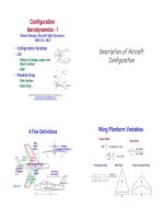
State Vector, 6 components!Nonlinear Dynamic Equations!
Fairchild-Republic A-10!
4
th
-Order Longitudinal
Equations of Motion!


u = f
1
= X / m − gsin
θ
− qw

w = f
2
= Z / m + gcos
θ
+ qu

q = f
3
= M / I
yy

θ
= f
4
= q
x
1
x
2
x
3
x

4
!
"
#
#
#
#
#
$
%
&
&
&
&
&
= x
Lon
4
=
u
w
q
θ
!
"
#
#
#
#
$

%
&
&
&
&
=
Axial Velocity, m/s
Vertical Velocity, m/s
Pitch Rate, rad/s
Pitch Angle, rad
!
"
#
#
#
#
#
$
%
&
&
&
&
&
State Vector, 4 components!
Nonlinear Dynamic Equations, neglecting range and altitude!
Fourth-Order Hybrid
Equations of Motion
Transform Longitudinal
Velocity Components"


u = f
1
= X / m − gsin
θ
− qw

w = f
2
= Z / m + gcos
θ
+ qu

q = f
3
= M / I
yy

θ
= f
4
= q


V = f
1
= T cos
α
+ i

( )
− D − mgsin
γ
$
%
&
'
m

γ
= f
2
= T sin
α
+ i
( )
+ L − mgcos
γ
$
%
&
'
mV

q = f
3
= M / I
yy

θ

= f
4
= q
x
1
x
2
x
3
x
4
!
"
#
#
#
#
#
$
%
&
&
&
&
&
=
u
w
q
θ

!
"
#
#
#
#
$
%
&
&
&
&
=
Axial Velocity
Vertical Velocity
Pitch Rate
Pitch Angle
!
"
#
#
#
#
#
$
%
&
&
&
&

&
x
1
x
2
x
3
x
4
!
"
#
#
#
#
#
$
%
&
&
&
&
&
=
V
γ
q
θ
!
"

#
#
#
#
#
$
%
&
&
&
&
&
=
Velocity
Flight Path Angle
Pitch Rate
Pitch Angle
!
"
#
#
#
#
#
$
%
&
&
&
&

&
i = Incidence angle of the thrust vector with respect to the centerline
•  Replace Cartesian body components of velocity by polar inertial components"
•  Replace X and Z by T, D, and L"
Hybrid Longitudinal
Equations of Motion"


V = f
1
= T cos
α
+ i
( )
− D − mgsin
γ
$
%
&
'
m

γ
= f
2
= T sin
α
+ i
( )
+ L − mgcos

γ
$
%
&
'
mV

q = f
3
= M / I
yy

θ
= f
4
= q


V = f
1
= T cos
α
+ i
( )
− D − mgsin
γ
$
%
&
'

m

γ
= f
2
= T sin
α
+ i
( )
+ L −mgcos
γ
$
%
&
'
mV

q = f
3
= M / I
yy

α
= f
4
=

θ
−


γ
= q −
1
mV
T sin
α
+ i
( )
+ L −mgcos
γ
$
%
&
'
x
1
x
2
x
3
x
4
!
"
#
#
#
#
#
$

%
&
&
&
&
&
=
V
γ
q
θ
!
"
#
#
#
#
#
$
%
&
&
&
&
&
=
Velocity
Flight Path Angle
Pitch Rate
Pitch Angle

!
"
#
#
#
#
#
$
%
&
&
&
&
&
x
1
x
2
x
3
x
4
!
"
#
#
#
#
#
$

%
&
&
&
&
&
=
V
γ
q
α
!
"
#
#
#
#
#
$
%
&
&
&
&
&
=
Velocity
Flight Path Angle
Pitch Rate
Angle of Attack

!
"
#
#
#
#
#
$
%
&
&
&
&
&
•  Replace pitch angle by angle of attack!
α
=
θ
−
γ
θ
=
α
+
γ
Why Transform Equations and
State Vector?"
•  Phugoid (long-period) mode is primarily
described by velocity and flight path angle"
•  Short-period mode is primarily described

by pitch rate and angle of attack"
x
1
x
2
x
3
x
4
!
"
#
#
#
#
#
$
%
&
&
&
&
&
=
V
γ
q
α
!
"

#
#
#
#
$
%
&
&
&
&
=
Velocity
Flight Path Angle
Pitch Rate
Angle of Attack
!
"
#
#
#
#
#
$
%
&
&
&
&
&
Why Transform Equations and State Vector?"

•  Hybrid linearized equations allow the
two modes to be examined separately"
F
Lon
=
F
Ph
F
SP
Ph
F
Ph
SP
F
SP
!
"
#
#
$
%
&
&
Effects of phugoid
perturbations on
phugoid motion"
Effects of phugoid
perturbations on
short-period motion"
Effects of short-

period perturbations
on phugoid motion"
Effects of short-period
perturbations on short-
period motion"
=
F
Ph
small
small F
SP
!
"
#
#
$
%
&
&
≈
F
Ph
0
0 F
SP
!
"
#
#
$

%
&
&
Nominal Equations of Motion in
Equilibrium (Trimmed Condition)"


x
N
(t ) = 0 = f[x
N
(t ),u
N
(t ),w
N
(t ),t ]


V
N
= 0 = f
1
= T cos
α
N
+ i
( )
− D − mgsin
γ
N

$
%
&
'
m

γ
N
= 0 = f
2
= T sin
α
N
+ i
( )
+ L − mg cos
γ
N
$
%
&
'
mV

q
N
= 0 = f
3
= M I
yy


α
N
= 0 = f
4
= q −
1
mV
T sin
α
N
+ i
( )
+ L − mg cos
γ
N
$
%
&
'
•  T, D, L, and M contain state, control, and disturbance effects"
x
N
T
=
V
N
γ
N
0

α
N
#
$
%
&
T
= constant
Linearized 
Equations of Motion
Sensitivity Matrices for
Longitudinal LTI Model"

Δ

x
Lon
(t ) = F
Lon
Δx
Lon
(t ) + G
Lon
Δu
Lon
(t ) + L
Lon
Δw
Lon
(t )

F =
∂
f
1
∂
V
∂
f
1
∂γ
∂
f
1
∂
q
∂
f
1
∂α
∂
f
2
∂
V
∂
f
2
∂γ
∂
f

2
∂
q
∂
f
2
∂α
∂
f
3
∂
V
∂
f
3
∂γ
∂
f
3
∂
q
∂
f
3
∂α
∂
f
4
∂
V

∂
f
4
∂γ
∂
f
4
∂
q
∂
f
4
∂α
$
%
&
&
&
&
&
&
&
&
&
&
&
'
(
)
)

)
)
)
)
)
)
)
)
)
G =
∂
f
1
∂δ
E
∂
f
1
∂δ
T
∂
f
1
∂δ
F
∂
f
2
∂δ
E

∂
f
2
∂δ
T
∂
f
2
∂δ
F
∂
f
3
∂δ
E
∂
f
3
∂δ
T
∂
f
3
∂δ
F
∂
f
4
∂δ
E

∂
f
4
∂δ
T
∂
f
4
∂δ
F
#
$
%
%
%
%
%
%
%
%
%
%
&
'
(
(
(
(
(
(

(
(
(
(
L =
∂
f
1
∂
V
wind
∂
f
1
∂α
wind
∂
f
2
∂
V
wind
∂
f
2
∂α
wind
∂
f
3

∂
V
wind
∂
f
3
∂α
wind
∂
f
4
∂
V
wind
∂
f
4
∂α
wind
#
$
%
%
%
%
%
%
%
%
%

%
%
&
'
(
(
(
(
(
(
(
(
(
(
(
Velocity Dynamics"


V = f
1
=
1
m
T cos
α
− D − mgsin
γ
[ ]
=
1

m
C
T
cos
α
ρ
V
2
2
S − C
D
ρ
V
2
2
S − mgsin
γ
%
&
'
(
)
*
•  Nonlinear equation"
Thrust incidence
angle neglected!
•  First row of linearized dynamic equation"

Δ


V (t) =
∂
f
1
∂
V
ΔV(t) +
∂
f
1
∂γ
Δ
γ
(t)+
∂
f
1
∂
q
Δq(t)+
∂
f
1
∂α
Δ
α
(t)
%
&
'

(
)
*
+
∂
f
1
∂δ
E
Δ
δ
E(t) +
∂
f
1
∂δ
T
Δ
δ
T (t)+
∂
f
1
∂δ
F
Δ
δ
F(t)
%
&

'
(
)
*
+
∂
f
1
∂
V
wind
ΔV
wind
+
∂
f
1
∂α
wind
Δ
α
wind
%
&
'
(
)
*
∂
f

1
∂
V
=
1
m
C
T
V
cos
α
N
− C
D
V
( )
ρ
V
N
2
2
S + C
T
N
cos
α
N
− C
D
N

( )
ρ
V
N
S
%
&
'
(
)
*
∂
f
1
∂γ
=
−1
m
mg cos
γ
N
[ ]
= −g cos
γ
N
∂
f
1
∂
q

=
−1
m
C
D
q
ρ
V
N
2
2
S
%
&
'
(
)
*
∂
f
1
∂α
=
−1
m
C
T
N
sin
α

N
+ C
D
α
( )
ρ
V
N
2
2
S
%
&
'
(
)
*
•  Coefficients in first row of F"
Sensitivity of Velocity Dynamics
to State Perturbations "
C
T
V
≡
∂
C
T
∂
V
C

D
V
≡
∂
C
D
∂
V
C
D
q
≡
∂
C
D
∂
q
C
D
α
≡
∂
C
D
∂α


V = C
T
cos

α
−C
D
( )
ρ
V
2
2
S − mgsin
γ
%
&
'
(
)
*
m
Sensitivity of Velocity Dynamics to
Control and Disturbance Perturbations "
∂
f
1
∂δ
E
=
−1
m
C
D
δ

E
ρ
V
N
2
2
S
%
&
'
(
)
*
∂
f
1
∂δ
T
=
1
m
C
T
δ
T
cos
α
N
ρ
V

N
2
2
S
%
&
'
(
)
*
∂
f
1
∂δ
F
=
−1
m
C
D
δ
F
ρ
V
N
2
2
S
%
&

'
(
)
*
•  Coefficients in first rows of G and L"
∂
f
1
∂
V
wind
= −
∂
f
1
∂
V
∂
f
1
∂α
wind
= −
∂
f
1
∂α
C
T
δ

T
≡
∂
C
T
∂δ
T
C
D
δ
E
≡
∂
C
D
∂δ
E
C
D
δ
F
≡
∂
C
D
∂δ
F
∂
f
2

∂
V
=
1
mV
N
C
T
V
sin
α
N
+ C
L
V
( )
ρ
V
N
2
2
S + C
T
N
sin
α
N
+ C
L
N

( )
ρ
V
N
S
$
%
&
'
(
)
−
1
mV
N
2
C
T
N
sin
α
N
+ C
L
N
( )
ρ
V
N
2

2
S − mg cos
γ
N
$
%
&
'
(
)
∂
f
2
∂γ
=
1
mV
N
mgsin
γ
N
[ ]
= gsin
γ
N
V
N
∂
f
2

∂
q
=
1
mV
N
C
L
q
ρ
V
N
2
2
S
$
%
&
'
(
)
∂
f
2
∂α
=
1
mV
N
C

T
N
cos
α
N
+ C
L
α
( )
ρ
V
N
2
2
S
$
%
&
'
(
)
•  Coefficients in second row of F"
Sensitivity of Flight Path Angle
Dynamics to State Perturbations "
•  Coefficients in second row of G and L in Supplemental Slide!
C
T
V
≡
∂

C
T
∂
V
C
L
V
≡
∂
C
L
∂
V
C
L
q
≡
∂
C
L
∂
q
C
L
α
≡
∂
C
L
∂α


γ
= C
T
sin
α
+ C
L
( )
ρ
V
2
2
S − mg cos
γ
%
&
'
(
)
*
mV
∂
f
3
∂
V
=
1

I
yy
C
m
V
ρ
V
N
2
2
Sc + C
m
N
ρ
V
N
Sc
#
$
%
&
'
(
∂
f
3
∂γ
= 0
∂
f

3
∂
q
=
1
I
yy
C
m
q
ρ
V
N
2
2
Sc
#
$
%
&
'
(
∂
f
3
∂α
=
1
I
yy

C
m
α
ρ
V
N
2
2
Sc
#
$
%
&
'
(
•  Coefficients in third row of F"
Sensitivity of Pitch Rate
Dynamics to State Perturbations "
C
m
V
≡
∂
C
m
∂
V
C
m
q

≡
∂
C
m
∂
q
C
m
α
≡
∂
C
m
∂α


q = C
m
ρ
V
2
2
( )
Sc I
yy
∂
f
4
∂
V

= −
∂
f
2
∂
V
∂
f
4
∂γ
= −
∂
f
2
∂γ
•  Coefficients in fourth row of F"
Sensitivity of Angle of Attack
Dynamics to State Perturbations "
∂
f
4
∂
q
= 1−
∂
f
2
∂
q
∂

f
4
∂α
= −
∂
f
2
∂α


α
=

θ
−

γ
= q −

γ
Dimensional Stability
and Control Derivatives
Dimensional Stability-Derivative
Notation"
!  Redefine force and moment symbols as acceleration symbols"
!  Dimensional stability derivatives portray acceleration
sensitivities to state perturbations"

Drag
mass (m)

⇒ D ∝

V
Lift
mass
⇒ L ∝V

γ
Moment
moment of inertia (I
yy
)
⇒ M ∝

q
Dimensional Stability-Derivative
Notation"

∂
f
1
∂
V
≡ −D
V

1
m
C
T

V
cos
α
N
−C
D
V
( )
ρ
V
N
2
2
S + C
T
N
cos
α
N
−C
D
N
( )
ρ
V
N
S
&
'
(

)
*
+

∂
f
2
∂α
≡
L
α
V
N

1
mV
N
C
T
N
cos
α
N
+ C
L
α
( )
ρ
V
N

2
2
S
%
&
'
(
)
*

∂
f
3
∂α
≡ M
α

1
I
yy
C
m
α
ρ
V
N
2
2
Sc
%

&
'
(
)
*
Thrust and drag effects are combined and represented by one symbol!
Thrust and lift effects are combined and represented by one symbol!
Longitudinal Stability Matrix"
F
Lon
=
F
Ph
F
SP
Ph
F
Ph
SP
F
SP
!
"
#
#
$
%
&
&
=

−D
V
−g cos
γ
N
−D
q
−D
α
L
V
V
N
g
V
N
sin
γ
N
L
q
V
N
L
α
V
N
M
V
0 M

q
M
α
−
L
V
V
N
−
g
V
N
sin
γ
N
1−
L
q
V
N
*
+
,
-
.
/
−
L
α
V

N
!
"
#
#
#
#
#
#
#
#
$
%
&
&
&
&
&
&
&
&
Effects of phugoid
perturbations on
phugoid motion"
Effects of phugoid
perturbations on
short-period motion"
Effects of short-period
perturbations on
phugoid motion"

Effects of short-period
perturbations on short-
period motion"
Primary Longitudinal Stability
Derivatives"

D
V

−1
m
C
T
V
−C
D
V
( )
ρ
V
N
2
2
S + C
T
N
−C
D
N
( )

ρ
V
N
S
#
$
%
&
'
(

Assuming
γ
N

α
N
 0

L
V
V
N

1
mV
N
C
L
V

ρ
V
N
2
2
S + C
L
N
ρ
V
N
S
"
#
$
%
&
'
−
1
mV
N
2
C
L
N
ρ
V
N
2

2
S − mg
"
#
$
%
&
'
M
q
=
1
I
yy
C
m
q
ρ
V
N
2
2
Sc
"
#
$
%
&
'
M

α
=
1
I
yy
C
m
α
ρ
V
N
2
2
Sc
#
$
%
&
'
(

L
α
V
N

1
mV
N
C

T
N
+ C
L
α
( )
ρ
V
N
2
2
S
#
$
%
&
'
(
Origins of Stability Effects
Velocity-Dependent Derivative
Definitions"
•  Air compressibility effects are a principal source of
velocity dependence"
C
D
M
≡
∂
C
D

∂
M
=
∂
C
D
∂
V / a
( )
= a
∂
C
D
∂
V
C
D
V
≡
∂
C
D
∂
V
=
1
a
#
$
%

&
'
(
C
D
M
C
L
V
≡
∂
C
L
∂
V
=
1
a
#
$
%
&
'
(
C
L
M
C
m
V

≡
∂
C
m
∂
V
=
1
a
#
$
%
&
'
(
C
m
M
C
D
M
≈ 0
C
D
M
> 0
C
D
M
< 0

a = Speed of Sound
M = Mach number =
V a
Pitch-Moment Coefficient
Sensitivity to Angle of Attack"
M
B
= C
m
q Sc ≈ C
m
o
+ C
m
q
q + C
m
α
α
( )
q Sc
C
m
α
≈ −C
N
α
net
h
cm

− h
cp
net
( )
≈ −C
L
α
net
h
cm
− h
cp
net
( )
= −C
L
α
net
x
cm
− x
cp
net
c
$
%
&
'
(
)

= C
m
α
wing
+ C
m
α
ht
Pitch-Rate Derivative Definitions"
•  Pitch rate derivatives are often expressed in terms of a
normalized pitch rate"
C
m
q
=
∂
C
m
∂
q
=
c
2V
N
"
#
$
%
&
'

C
m
ˆ
q
C
m
ˆ
q
=
∂
C
m
∂
ˆ
q
=
∂
C
m
∂
qc
2V
N
( )
=
2V
N
c
"
#

$
%
&
'
C
m
q
ˆ
q =
q
c
2V
N
M
q
=
∂
M
∂
q
= C
m
q
ρ
V
N
2
2
( )
Sc = C

m
ˆ
q
c
2V
N
#
$
%
&
'
(
ρ
V
N
2
2
#
$
%
&
'
(
S
c = C
m
ˆ
q
ρ
V

N
Sc
2
4
#
$
%
&
'
(
often tabulated! used in pitch-rate equation!
M
B
= C
m
q Sc ≈ C
m
o
+ C
m
q
q + C
m
α
α
( )
q Sc
≈ C
m
o

+
∂C
m
∂q
q + C
m
α
α
$
%
&
'
(
)
q Sc
•  Pitch acceleration sensitivity to pitch rate"
Pitch-Rate Derivative Definitions"
•  Pitch rate derivatives are often expressed
in terms of a normalized pitch rate"
C
m
q
=
∂
C
m
∂
q
=
c

2V
N
"
#
$
%
&
'
C
m
ˆ
q
C
m
ˆ
q
=
∂
C
m
∂
ˆ
q
=
∂
C
m
∂
qc
2V

N
( )
=
2V
N
c
"
#
$
%
&
'
C
m
q
ˆ
q =
q
c
2V
N
M
B
= C
m
q Sc ≈ C
m
o
+ C
m

q
q + C
m
α
α
( )
q Sc
≈ C
m
o
+
∂C
m
∂q
q + C
m
α
α
$
%
&
'
(
)
q Sc
•  Then"
•  But dynamic equations require ∂C
m
/∂q "
Angle of Attack Distribution

Due to Pitch Rate"
•  Aircraft pitching at a constant rate, q rad/s, produces a normal
velocity distribution along x"
Δw = −qΔx
Δ
α
=
Δw
V
N
=
−qΔx
V
N
•  Corresponding angle of attack distribution"
Δ
α
ht
=
ql
ht
V
N
•  Angle of attack perturbation at tail center of pressure"
€
l
ht
= horizontal tail distance from c.m.
Horizontal Tail Lift
Due to Pitch Rate"

•  Incremental tail lift due to pitch rate, referenced to tail area, S
ht
"
•  Lift coefficient sensitivity to pitch rate referenced to wing area"
ΔL
ht
= ΔC
L
ht
( )
ht
1
2
ρ
V
N
2
S
ht
C
L
q
ht
≡
∂
ΔC
L
ht
( )
aircraft

∂
q
=
∂
C
L
ht
∂α
%
&
'
(
)
*
aircraft
l
ht
V
N
%
&
'
(
)
*
ΔC
L
ht
( )
aircraft

= ΔC
L
ht
( )
ht
S
ht
S
"
#
$
%
&
'
=
∂
C
L
ht
∂α
"
#
$
%
&
'
aircraft
Δ
α
*

+
,
,
-
.
/
/
=
∂
C
L
ht
∂α
"
#
$
%
&
'
aircraft
ql
ht
V
N
"
#
$
%
&
'

•  Incremental tail lift coefficient due to pitch rate, referenced to
wing area, S"
Moment Coefficient
Sensitivity to Pitch Rate of
the Horizontal Tail"
•  Differential pitch moment due to pitch rate"
∂
ΔM
ht
∂
q
= C
m
q
ht
1
2
ρ
V
N
2
Sc = −C
L
q
ht
l
ht
V
N
%

&
'
(
)
*
1
2
ρ
V
N
2
Sc
= −
∂
C
L
ht
∂α
%
&
'
(
)
*
aircraft
l
ht
V
N
%

&
'
(
)
*
,
-
.
.
/
0
1
1
l
ht
c
%
&
'
(
)
*
1
2
ρ
V
N
2
Sc
C

m
q
ht
= −
∂
C
L
ht
∂α
l
ht
V
N
$
%
&
'
(
)
l
ht
c
$
%
&
'
(
)
= −
∂

C
L
ht
∂α
l
ht
c
$
%
&
'
(
)
2
c
V
N
$
%
&
'
(
)
•  Coefficient derivative with respect to pitch rate"
•  Coefficient derivative with respect to normalized pitch rate
is insensitive to velocity"
C
m
ˆ
q

ht
=
∂
C
m
ht
∂
ˆ
q
=
∂
C
m
ht
∂
qc
2V
N
( )
= −2
∂
C
L
ht
∂α
l
ht
c
$
%

&
'
(
)
2
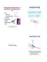
Comparison of Fourth-
and Second-Order
Dynamic Models
•  0 - 100 sec"
•  Reveals Phugoid Mode"
4
th
-Order Initial-Condition
Responses of Business Jet
at Two Time Scales"
•  0 - 6 sec"
•  Reveals Short-Period Mode"
•  Plotted over different periods of time"
–  4 initial conditions"
Second-Order Models of
Longitudinal Motion"
•  2
nd
-Order Approximate Phugoid Equation"

Δ

x
Ph
=

Δ

V
Δ

γ
#
$
%
%
&
'
(
(
≈
−D
V
−gcos
γ
N
L
V
V
N
g
V
N
sin
γ
N

#
$
%
%
%
&
'
(
(
(
ΔV
Δ
γ
#
$
%
%
&
'
(
(
+
T
δ
T
L
δ
T
V
N

#
$
%
%
%
&
'
(
(
(
Δ
δ
T +
−D
V
L
V
V
N
#
$
%
%
%
&
'
(
(
(
ΔV

wind

Δ

x
SP
=
Δ

q
Δ

α
#
$
%
%
&
'
(
(
≈
M
q
M
α
1 −
L
q
V

N
+
,
-
.
/
0
−
L
α
V
N
#
$
%
%
%
&
'
(
(
(
Δq
Δ
α
#
$
%
%
&

'
(
(
+
M
δ
E
−L
δ
E
V
N
#
$
%
%
%
&
'
(
(
(
Δ
δ
E +
M
α
−L
α
V

N
#
$
%
%
%
&
'
(
(
(
Δ
α
wind
•  2
nd
-Order Approximate Short-Period Equation"
•  Assume off-diagonal blocks of (4 x 4)
stability matrix are negligible"
F
Lon
=
F
Ph
~ 0
~ 0 F
SP
!
"
#

#
$
%
&
&
•  Phugoid Time Scale" •  Short-Period Time Scale"
•  Full and approximate linear models"
Comparison of Bizjet Fourth- and
Second-Order Model Responses"
•  Fourth
Order"
•  Second
Order"
•  Approximations are very close to 4
th
-order values
because natural frequencies are widely separated"
Comparison of Bizjet Fourth- and
Second-Order Models and Eigenvalues"
Fourth-Order Model
F = G = Eigenvalue Damping Freq. (rad/s)

-0.0185 -9.8067 0 0 0 4.6645 -8.43e-03 + 1.24e-01j 6.78E-02 1.24E-01
0.0019 0 0 1.2709 0 0 -8.43e-03 - 1.24e-01j 6.78E-02 1.24E-01
0 0 -1.2794 -7.9856 -9.069 0
-1.28e+00 + 2.83e+00j
4.11E-01 3.10E+00
-0.0019 0 1 -1.2709 0 0
-1.28e+00 - 2.83e+00j
4.11E-01 3.10E+00

Phugoid Approximation
F = G = Eigenvalue Damping Freq. (rad/s)

-0.0185 -9.8067 4.6645 -9.25e-03 + 1.36e-01j 6.78E-02 1.37E-01
0.0019 0 0 -9.25e-03 - 1.36e-01j 6.78E-02 1.37E-01
Short-Period Approximation
F = G = Eigenvalue Damping Freq. (rad/s)

-1.2794 -7.9856 -9.069
-1.28e+00 + 2.83e+00j
4.11E-01 3.10E+00
1 -1.2709 0
-1.28e+00 - 2.83e+00j
4.11E-01 3.10E+00
Approximate Phugoid Roots "
•  Approximate Phugoid Equation (
!
N
= 0)"

Δ

x
Ph
=
Δ

V
Δ


γ
#
$
%
%
&
'
(
(
≈
−D
V
−g
L
V
V
N
0
#
$
%
%
%
&
'
(
(
(
ΔV
Δ

γ
#
$
%
%
&
'
(
(
+
T
δ
T
L
δ
T
V
N
#
$
%
%
%
&
'
(
(
(
Δ
δ

T
•  Characteristic polynomial"
sI − F
Ph
= det sI − F
Ph
( )
≡ Δ(s) = s
2
+ D
V
s + gL
V
/ V
N
= s
2
+ 2
ζω
n
s +
ω
n
2
ω
n
= gL
V
/ V
N

ζ
=
D
V
2 gL
V
/ V
N
•  Natural frequency and
damping ratio"
ω
n
≈ 2
g
V
N
; T = 2
π
/
ω
n
ζ
≈
1
2
L / D
( )
N
•  Neglecting
compressibility effects"

Effect of Airspeed and L/D on Approximate
Phugoid Natural Frequency, Period, and
Damping Ratio "
ω
n
≈ 2
g
V
N
≈ 13.87 /V
N
(m / s)
ζ
≈
1
2
L / D
( )
N
Velocity
Natural
Frequency
Period L/D
Damping
Ratio
m/s rad/s sec
50 0.28 23 5 0.14
100 0.14 45 10 0.07
200 0.07 90 20 0.035
400 0.035 180 40 0.018

Neglecting
compressibility effects"
Period, T = 2
π
/
ω
n
≈ 0.45V
N
sec
Approximate Phugoid Response to
a 10% Thrust Increase "
•  What is the steady-state response?"
Approximate Short-Period Roots "
•  Approximate Short-Period Equation (L
q
= 0)"
•  Characteristic polynomial"
•  Natural frequency and damping ratio"

Δ

x
SP
=
Δ

q
Δ


α
#
$
%
%
&
'
(
(
≈
M
q
M
α
1 −
L
α
V
N
#
$
%
%
%
&
'
(
(
(
Δq

Δ
α
#
$
%
%
&
'
(
(
+
M
δ
E
−L
δ
E
V
N
#
$
%
%
%
&
'
(
(
(
Δ

δ
E
Δ(s) = s
2
+
L
α
V
N
− M
q
$
%
&
'
(
)
s − M
α
+ M
q
L
α
V
N
$
%
&
'
(

)
= s
2
+ 2
ζω
n
s +
ω
n
2
ω
n
= − M
α
+ M
q
L
α
V
N
$
%
&
'
(
)
;
ζ
=
L

α
V
N
− M
q
$
%
&
'
(
)
2 − M
α
+ M
q
L
α
V
N
$
%
&
'
(
)
Generally,
L
α
> 0
M

α
< 0
M
q
< 0
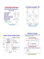
Approximate Short-Period Response
to a 0.1-Rad Pitch Control Step Input "
Pitch Rate, rad/s! Angle of Attack, rad!
Normal Load Factor Response to a
0.1-Rad Pitch Control Step Input "
Normal Load Factor, g

s at c.m.!
Aft Pitch Control (Elevator)!
Normal Load Factor, g

s at c.m.!
Forward Pitch Control (Canard)!

n
z
=
V
N
g
Δ

α
− Δq
( )

=
V
N
g
L
α
V
N
Δ
α
+
L
δ
E
V
N
Δ
δ
E
%
&
'
(
)
*
•  Normal load factor at the center of mass"
•  Pilot focuses on normal load factor during rapid maneuvering"
Grumman X-29!
Next Time:
Lateral-Directional Dynamics


Reading
Flight Dynamics, 96-101,
574-582, 587-591
Virtual Textbook, Part 12
Supplemental
Material
Flight Path Angle Dynamics"
•  Second row of linearized equation"


γ
= f
2
=
1
mV
T sin
α
+ L − mgcos
γ
[ ]
=
1
mV
C
T
sin
α
ρ

V
2
2
S + C
L
ρ
V
2
2
S − mg cos
γ
%
&
'
(
)
*
•  Nonlinear equation"

Δ

γ
(t) =
∂
f
2
∂
V
ΔV(t) +
∂

f
2
∂γ
Δ
γ
(t) +
∂
f
2
∂
q
Δq(t) +
∂
f
2
∂α
Δ
α
(t)
%
&
'
(
)
*
+
∂
f
2
∂δ

E
Δ
δ
E(t) +
∂
f
2
∂δ
T
Δ
δ
T (t) +
∂
f
2
∂δ
F
Δ
δ
F(t)
%
&
'
(
)
*
+
∂
f
2

∂
V
wind
ΔV
wind
+
∂
f
2
∂α
wind
Δ
α
wind
%
&
'
(
)
*
Pitch Rate Dynamics"


q = f
3
=
M
I
yy
=

C
m
ρ
V
2
2
( )
Sc
I
yy
C
m
may include thrust
as well as
aerodynamic effects!
•  Nonlinear equation"
•  Third row of linearized equation"

Δ

q(t) =
∂
f
3
∂
V
ΔV(t) +
∂
f
3

∂γ
Δ
γ
(t) +
∂
f
3
∂
q
Δq(t) +
∂
f
3
∂α
Δ
α
(t)
%
&
'
(
)
*
+
∂
f
3
∂δ
E
Δ

δ
E(t) +
∂
f
3
∂δ
T
Δ
δ
T (t) +
∂
f
3
∂δ
F
Δ
δ
F(t)
%
&
'
(
)
*
+
∂
f
3
∂
V

wind
ΔV
wind
+
∂
f
3
∂α
wind
Δ
α
wind
%
&
'
(
)
*
Angle of Attack Dynamics"


α
= f
4
=

θ
−

γ

= q −
1
mV
T sin
α
+ L − mg cos
γ
[ ]
•  Nonlinear equation"
•  Fourth row of linearized equation"

Δ

α
(t) =
∂
f
4
∂
V
ΔV(t) +
∂
f
4
∂γ
Δ
γ
(t) +
∂
f

4
∂
q
Δq(t) +
∂
f
4
∂α
Δ
α
(t)
%
&
'
(
)
*
+
∂
f
4
∂δ
E
Δ
δ
E(t) +
∂
f
4
∂δ

T
Δ
δ
T (t) +
∂
f
4
∂δ
F
Δ
δ
F(t)
%
&
'
(
)
*
+
∂
f
4
∂
V
wind
ΔV
wind
+
∂
f

4
∂α
wind
Δ
α
wind
%
&
'
(
)
*
Elements of the Stability Matrix"
∂
f
1
∂
V
≡ − D
V
;
∂
f
1
∂γ
= −gcos
γ
N
;
∂

f
1
∂
q
≡ − D
q
;
∂
f
1
∂α
≡ − D
α
∂
f
2
∂
V
≡
L
V
V
N
;
∂
f
2
∂γ
=
g

V
N
sin
γ
N
;
∂
f
2
∂
q
≡
L
q
V
N
;
∂
f
2
∂α
≡
L
α
V
N
∂
f
3
∂

V
≡ M
V
;
∂
f
3
∂γ
= 0;
∂
f
3
∂
q
≡ M
q
;
∂
f
3
∂α
≡ M
α
∂
f
4
∂
V
≡ −
L

V
V
N
;
∂
f
4
∂γ
= −
g
V
N
sin
γ
N
;
∂
f
4
∂
q
≡ 1−
L
q
V
N
;
∂
f
4

∂α
≡ −
L
α
V
N
•  Stability derivatives portray acceleration
sensitivities to state perturbations"
∂
f
2
∂δ
E
=
1
mV
N
C
L
δ
E
ρ
V
N
2
2
S
$
%
&

'
(
)
∂
f
2
∂δ
T
=
1
mV
N
C
T
δ
T
sin
α
N
ρ
V
N
2
2
S
$
%
&
'
(

)
∂
f
2
∂δ
F
=
1
mV
N
C
L
δ
F
ρ
V
N
2
2
S
$
%
&
'
(
)
∂
f
2
∂

V
wind
= −
∂
f
2
∂
V
∂
f
2
∂α
wind
= −
∂
f
2
∂α
Control and Disturbance Sensitivities in
Flight Path Angle, Pitch Rate, and Angle-of-
Attack Dynamics"
∂
f
3
∂δ
E
=
1
I
yy

C
m
δ
E
ρ
V
N
2
2
Sc
$
%
&
'
(
)
∂
f
3
∂δ
T
=
1
I
yy
C
m
δ
T
ρ

V
N
2
2
Sc
$
%
&
'
(
)
∂
f
3
∂δ
F
=
1
I
yy
C
m
δ
F
ρ
V
N
2
2
Sc

$
%
&
'
(
)
∂
f
3
∂
V
wind
= −
∂
f
3
∂
V
∂
f
3
∂α
wind
= −
∂
f
3
∂α
∂
f

4
∂δ
E
= −
∂
f
2
∂δ
E
∂
f
4
∂δ
T
= −
∂
f
2
∂δ
T
∂
f
4
∂δ
F
= −
∂
f
2
∂δ

F
∂
f
4
∂
V
wind
=
∂
f
2
∂
V
∂
f
3
∂α
wind
=
∂
f
2
∂α
Horizontal Tail Lift Sensitivity
to Angle of Attack"
C
L
α
ht
( )

aircraft
=
V
tail
V
N
"
#
$
%
&
'
2
1−
∂ε
∂α
"
#
$
%
&
'
η
elas
S
ht
S
"
#
$

%
&
'
C
L
α
ht
( )
ε
= Wing downwash angle at the
tail
!
V
Tail
= Airspeed at vertical tail;
scrubbing lowers V
Tail
,
propeller slipstream increases
V
Tail!
η
elas
= Aeroelastic correction
factor
!
Wing Lift and Moment Coefficient
Sensitivity to Pitch Rate"
•  Straight-wing incompressible flow estimate (Etkin)"
C

L
ˆ
q
wing
= −2C
L
α
wing
h
cm
− 0.75
( )
C
m
ˆ
q
wing
= −2C
L
α
wing
h
cm
− 0.5
( )
2
•  Straight-wing supersonic flow estimate (Etkin)"
C
L
ˆ

q
wing
= −2C
L
α
wing
h
cm
− 0.5
( )
C
m
ˆ
q
wing
= −
2
3 M
2
− 1
− 2C
L
α
wing
h
cm
− 0.5
( )
2
•  Triangular-wing estimate (Bryson, Nielsen)"

C
L
ˆ
q
wing
= −
2
π
3
C
L
α
wing
C
m
ˆ
q
wing
= −
π
3AR
Control- and Disturbance-
Effect Matrices"
•  Control-effect derivatives portray acceleration
sensitivities to control input perturbations"
•  Disturbance-effect derivatives portray acceleration sensitivities
to disturbance input perturbations"
G
Lon
=

−D
δ
E
T
δ
T
−D
δ
F
L
δ
E
/ V
N
L
δ
T
/ V
N
L
δ
F
/ V
N
M
δ
E
M
δ
T

M
δ
F
−L
δ
E
/ V
N
−L
δ
T
/ V
N
−L
δ
F
/ V
N
#
$
%
%
%
%
%
&
'
(
(
(

(
(
L
Lon
=
−D
V
wind
−D
α
wind
L
V
wind
/ V
N
L
α
wind
/ V
N
M
V
wind
M
α
wind
−L
V
wind

/ V
N
−L
α
wind
/ V
N
#
$
%
%
%
%
%
%
&
'
(
(
(
(
(
(
Primary Longitudinal
Control Derivatives"

D
δ
T


−1
m
C
T
δ
T
ρ
V
N
2
2
S
$
%
&
'
(
)
L
δ
F
V
N

1
mV
N
C
L
δ

F
ρ
V
N
2
2
S
$
%
&
'
(
)
M
δ
E
=
1
I
yy
C
m
δ
E
ρ
V
N
2
2
Sc

$
%
&
'
(
)
Effects of Airspeed, Altitude, Mass, and Moment of
Inertia on Fighter Aircraft Short Period"
Airspeed Altitude
Natural
Frequency
Period
Damping
Ratio
m/s m rad/s sec -
122 2235 2.36 2.67 0.39
152 6095 2.3 2.74 0.31
213 11915 2.24 2.8 0.23
274 16260 2.18 2.88 0.18
Mass
Variation
Natural
Frequency
Period
Damping
Ratio
% rad/s sec -
-50 2.4 2.62 0.44
0 2.3 2.74 0.31
50 2.26 2.78 0.26

Moment of
Inertia
Variation
Natural
Frequency
Period
Damping
Ratio
% rad/s sec -
-50 3.25 1.94 0.33
0 2.3 2.74 0.31
50 1.87 3.35 0.31
Airspeed
Dynamic
Pressure
Angle of
Attack
Natural
Frequency
Period
Damping
Ratio
m/s P deg rad/s sec -
91 2540 14.6 1.34 4.7 0.3
152 7040 5.8 2.3 2.74 0.31
213 13790 3.2 3.21 1.96 0.3
274 22790 2.2 3.84 1.64 0.3
Airspeed variation at constant altitude!
Altitude variation with constant dynamic pressure!
Mass variation at constant altitude!

Moment of inertia variation at constant altitude!
Flight Motions "
Dornier Do-128 Short-Period Demonstration"
/>"
Simulator Demonstration of "
Short-Period Response to Elevator Deflection"
/>"
Dornier Do-128D!
•  Rapid damping"
•  Pitch angle and rate response"
•  Flight path angle reoriented by difference
between pitch angle and angle of attack"
Dornier Do-128 Phugoid Demonstration"
/>"