Aircraft Flight Dynamics Robert F. Stengel Lecture14 RootLocus Analysis of Parameter Variations
Bạn đang xem bản rút gọn của tài liệu. Xem và tải ngay bản đầy đủ của tài liệu tại đây (1.04 MB, 11 trang )
Root Locus Analysis of
Parameter Variations
Robert Stengel, Aircraft Flight Dynamics
MAE 331, 2012"
• Effects of system parameter
variations on modes of motion"
• Root locus analysis"
– Evanss rules for construction"
– Application to longitudinal
dynamic models"
Copyright 2012 by Robert Stengel. All rights reserved. For educational use only.!
/>!
/>!
Characteristic Equation: A Critical
Component of the Response’s
Laplace Transform "
sI − F
[ ]
−1
=
Adj sI − F
( )
sI − F
=
C
T
s
( )
sI − F
(n × n)
1×1
( )
• Characteristic equation defines the modes of motion!
sI − F = Δ(s) = s
n
+ a
n −1
s
n −1
+ + a
1
s + a
0
= s −
λ
1
( )
s −
λ
2
( )
( )
s −
λ
n
( )
= 0
Δx(s) = sI − F
[ ]
−1
Δx( 0) + G Δu(s) + LΔw(s)
[ ]
• Recall: s is a complex variable!
s =
σ
+ j
ω
Real Roots of the Dynamic System "
Δ(s) = s −
λ
1
( )
s −
λ
2
( )
( )
s −
λ
n
( )
= 0
• Roots are solutions of the
characteristic equation"
λ
i
=
µ
i
(Real number)
x t
( )
= x 0
( )
e
µ
t
• Real roots"
– are confined to the real axis"
– represent convergent or divergent
time response"
– time constant,
τ
= –1/
λ
= –1/
µ
, sec
#
s Plane =
σ
+ j
ω
( )
Plane
Complex Roots of the Dynamic System "
€
δ
= cos
−1
ζ
• Complex roots"
– occur only in complex-conjugate pairs"
– represent oscillatory modes"
– natural frequency,
ω
n
, and damping ratio,
ζ
, as shown"
s Plane =
σ
+ j
ω
( )
Plane
λ
1
=
µ
1
+ j
ν
1
= −
ζω
n
+ j
ω
n
1−
ζ
2
– time constant = –1/μ = 1/ζω
n
"
Stable" Unstable"
– decay of exponential time-"
response envelope"
λ
2
=
µ
2
+ j
ν
2
=
µ
1
− j
ν
1
=
λ
1
*
= −
ζω
n
− j
ω
n
1−
ζ
2
Complex Roots, Damping Ratio,
and Damped Natural Frequency "
s −
λ
1
( )
s −
λ
1
*
( )
= s −
µ
1
+ j
ν
1
( )
$
%
&
'
s −
µ
1
− j
ν
1
( )
$
%
&
'
= s
2
−
µ
1
− j
ν
1
( )
+
µ
1
+ j
ν
1
( )
$
%
&
'
s +
µ
1
− j
ν
1
( )
µ
1
+ j
ν
1
( )
= s
2
− 2
µ
1
s +
µ
1
2
+
ν
1
2
( )
s
2
+ 2
ζω
n
s +
ω
n
2
µ
1
= −
ζω
n
= −1 Time constant
ν
1
=
ω
n
1−
ζ
2
ω
n
damped
= Damped natural frequency
x
1
t
( )
= Ae
−
ζω
n
t
sin
ω
n
1−
ζ
2
t +
ϕ
%
&
'
(
x
2
t
( )
= Ae
−
ζω
n
t
ω
n
1−
ζ
2
%
&
'
(
cos
ω
n
1−
ζ
2
t +
ϕ
%
&
'
(
Identical exponentially
decaying envelopes for
both displacement and rate"
Corresponding Second-Order
Initial Condition Response"
General form of response"
Multi-Modal LTI Responses Superpose
Individual Modal Responses"
• With distinct roots, (n = 4)
for example, partial
fraction expansion for
each state element is
(Flight Dynamics, p. 325)
"
Δx
i
s
( )
=
d
1
i
s −
λ
1
( )
+
d
2
i
s −
λ
2
( )
+
d
2
i
s −
λ
3
( )
+
d
2
i
s −
λ
4
( )
• Corresponding 4
th
-order time response is"
Δx
i
t
( )
= d
1
i
e
λ
1
t
+ d
2
i
e
λ
2
t
+ d
3
i
e
λ
3
t
+ d
4
i
e
λ
4
t
• Details in next lecture"
Evanss Rules for
Root Locus Analysis
Root Locus Example: "
4
th-
Order Longitudinal
Characteristic Equation"
Δ
Lon
(s) = s
4
+ a
3
s
3
+ a
2
s
2
+ a
1
s + a
0
= s
4
+ D
V
+
L
α
V
N
− M
q
( )
s
3
+ g − D
α
( )
L
V
V
N
+ D
V
L
α
V
N
− M
q
( )
− M
q
L
α
V
N
− M
α
$
%
&
'
(
)
s
2
+ M
q
D
α
− g
( )
L
V
V
N
− D
V
L
α
V
N
$
%
&
'
(
)
+ D
α
M
V
− D
V
M
α
{ }
s
+ g M
V
L
α
V
N
− M
α
L
V
V
N
( )
= 0
Δ
Lon
(s) = s
2
+ 2
ζω
n
s +
ω
n
2
( )
Ph
s
2
+ 2
ζω
n
s +
ω
n
2
( )
SP
• Typically factors into oscillatory phugoid and short-period modes
"
€
with L
q
= D
q
= 0
Root Locus Analysis of
Parametric Effects on
Aircraft Dynamics
"
• Parametric variations alter
eigenvalues of F"
• Graphical technique for
finding the roots with a
new parameter value"
Locus: the set of all points whose
location is determined by stated
conditions"
s Plane!
Phugoid "
Roots"
Short Period"
Root"
Short Period"
Root"
Example: How do the roots vary when
we change pitch-rate damping, M
q
?"
Δ
Lon
(s) = s
4
+ D
V
+
L
α
V
N
− M
q
( )
s
3
+ g − D
α
( )
L
V
V
N
+ D
V
L
α
V
N
− M
q
( )
− M
q
L
α
V
N
− M
α
$
%
&
'
(
)
s
2
+ M
q
D
α
− g
( )
L
V
V
N
− D
V
L
α
V
N
$
%
&
'
(
)
+ D
α
M
V
− D
V
M
α
{ }
s
+ g M
V
L
α
V
N
− M
α
L
V
V
N
( )
= 0
• M
q
could be changed by"
– Variation in aircraft aerodynamic configuration"
– Effect of feedback control, i.e., control of
pitching moment (via elevator) that is
proportional to pitch rate"
Effect of Parameter
Variations on Root
Location "
• Let root locus gain = k = a
i
(just a notation change)
"
– Option 1: Vary k and calculate roots for each new value"
– Option 2: Apply Evanss Rules of Root Locus Construction"
Walter R. Evans"
Δ
Lon
(s) = s
4
+ a
3
s
3
+ a
2
s
2
+ a
1
s + a
0
= s −
λ
1
( )
s −
λ
2
( )
s −
λ
3
( )
s −
λ
4
( )
= s −
λ
1
( )
s −
λ
1
*
( )
s −
λ
3
( )
s −
λ
3
*
( )
= s
2
+ 2
ζ
P
ω
n
P
s +
ω
n
P
2
( )
s
2
+ 2
ζ
SP
ω
n
SP
s +
ω
n
SP
2
( )
= 0
Effect of a
0
Variation on
Longitudinal Root Location "
• Example: Root locus gain, k = a
0
!
where
d(s) = s
4
+ a
3
s
3
+ a
2
s
2
+ a
1
s
= s −
λ
'
1
( )
s −
λ
'
2
( )
s −
λ
'
3
( )
s −
λ
'
4
( )
n(s) = 1
Δ
Lon
(s) = s
4
+ a
3
s
3
+ a
2
s
2
+ a
1
s
"
#
$
%
+ k
[ ]
≡ d(s)+ kn(s)
= s −
λ
1
( )
s −
λ
2
( )
s −
λ
3
( )
s −
λ
4
( )
= 0
d s
( )
: Polynomial in s
n s
( )
: Polynomial in s
• Example: Root locus gain, k = a
1
!
where
d(s) = s
4
+ a
3
s
3
+ a
2
s
2
+ a
0
= s −
λ
'
1
( )
s −
λ
'
2
( )
s −
λ
'
3
( )
s −
λ
'
4
( )
n(s) = s
Δ
Lon
(s) = s
4
+ a
3
s
3
+ a
2
s
2
+ ks + a
0
≡ d(s)+ kn(s)
= s −
λ
1
( )
s −
λ
2
( )
s −
λ
3
( )
s −
λ
4
( )
= 0
Effect of a
1
Variation on
Longitudinal Root Location "
Three Equivalent Equations
for Defining Roots "
1 + k
n(s)
d(s)
= 0
k
n(s)
d(s)
= −1 = (1)e
− j
π
(rad )
= (1)e
− j180(deg)
d(s) + k n(s) = 0
Longitudinal Equation Example"
• Original 4
th
-order polynomial!
Δ
Lon
(s) = s
4
+ 2.57s
3
+ 9.68s
2
+ 0.202s + 0.145
= s
2
+ 2 0.0678
( )
0.124s + 0.124
( )
2
"
#
$
%
s
2
+ 2 0.411
( )
3.1s + 3.1
( )
2
"
#
$
%
= 0
Δ
Lon
(s) = s
4
+ a
3
s
3
+ a
2
s
2
+ a
1
s + a
0
= s −
λ
1
( )
s −
λ
2
( )
s −
λ
3
( )
s −
λ
4
( )
= s −
λ
1
( )
s −
λ
1
*
( )
s −
λ
3
( )
s −
λ
3
*
( )
= s
2
+ 2
ζ
P
ω
n
P
s +
ω
n
P
2
( )
s
2
+ 2
ζ
SP
ω
n
SP
s +
ω
n
SP
2
( )
= 0
• Typical flight condition!
Phugoid" Short Period"
Example: Effect of a
0
Variation"
Δ(s) = s
4
+ a
3
s
3
+ a
2
s
2
+ a
1
s + a
0
= s
4
+ a
3
s
3
+ a
2
s
2
+ a
1
s
( )
+ k
= s s
3
+ a
3
s
2
+ a
2
s + a
1
( )
+ k
= s s + 0.21
( )
s
2
+ 2.55s +9.62
"
#
$
%
+ k
k
s s + 0.21
( )
s
2
+ 2.55s + 9.62
!
"
#
$
= −1
• Example: k = a
0
!
• Original 4
th
-order polynomial!
Δ
Lon
(s) = s
4
+ 2.57s
3
+ 9.68s
2
+ 0.202s + 0.145 = 0
• Rearrange:!
ks
s
2
− 0.00041s + 0.015
"
#
$
%
s
2
+ 2.57s + 9.67
"
#
$
%
= −1
• Example: k = a
1
!
Δ(s) = s
4
+ a
3
s
3
+ a
2
s
2
+ a
1
s +a
0
= s
4
+ a
3
s
3
+ a
2
s
2
+ ks + a
0
= s
4
+ a
3
s
3
+ a
2
s
2
+ a
0
( )
+ ks
= s
2
− 0.00041s + 0.015
#
$
%
&
s
2
+ 2.57 s + 9.67
#
$
%
&
+ ks
Example: Effect of a
1
Variation"
• Rearrange:!
The Root Locus Criterion"
• All points on the locus of roots must satisfy the equation
k[n(s)/d(s)] = –1"
• Phase angle(–1) = ±180 deg"
k = a
0
: k
n(s)
d(s)
= k
1
s
4
+ a
3
s
3
+ a
2
s
2
+ a
1
s
= −1
k = a
1
: k
n(s)
d(s)
= k
s
s
4
+ a
3
s
3
+ a
2
s
2
+ a
0
= −1
= k
s − 0
( )
s
4
+ a
3
s
3
+ a
2
s
2
+ a
0
= −1
• Number of roots = 4"
• Number of zeros = 0"
• (n – q) = 4"
• Number of roots = 4"
• Number of zeros = 1"
• (n – q) = 3"
• Number of roots (or poles) of the denominator = n"
• Number of zeros of the numerator = q"
Spirule"
Origins of Roots (for k = 0)"
Δ(s) = d(s) + kn (s)
k → 0
# →## d(s)
• Origins of the roots are the Poles of d(s)"
Destinations of Roots (for k -> ±∞) "
• q roots go to the zeros of n(s)"
d(s)+ kn(s)
k
=
d(s)
k
+ n(s)
k→∞
# →## n(s) = s − z
1
( )
s − z
2
( )
No zeros when k = a
0
" One zero at origin when k = a
1
"
Destinations of Roots (for k -> ±∞) "
d(s)+ kn(s)
n(s)
!
"
#
$
%
&
=
d(s)
n(s)
+ k
!
"
#
$
%
&
k→±R→±∞
) →)))
s
n
s
q
+ k
!
"
#
$
%
&
→ s
n−q
( )
± R →±∞
• (n – q) roots go to infinite radius from the origin"
R(+)"
R(–)"
s
n−q
( )
= Re
− j180°
→ ∞ or Re
− j 360°
→ −∞
s = R
1 n−q
( )
e
− j180° n−q
( )
→ ∞ or R
1 n−q
( )
e
− j 360° n−q
( )
→ −∞
• Asymptotes of the root loci are described by"
• Magnitudes of roots are the same for given k"
• Angles from the origin are different"
Destinations of Roots (for k -> ±∞) "
4 roots to infinite radius"
3 roots to infinite radius"
(n – q) Roots Approach Asymptotes
as k –> ±∞"
θ
(rad) =
π
+ 2m
π
n − q
, m = 0,1, ,(n − q) − 1
θ
(rad) =
2m
π
n − q
, m = 0,1, ,(n − q) − 1
• Asymptote angles for positive k"
• Asymptote angles for negative k"
Origin of Asymptotes =
Center of Gravity"
"c.g." =
σ
λ
i
−
σ
z
j
j =1
q
∑
i =1
n
∑
n − q
Root Locus on Real Axis"
• Locus on real axis"
– k > 0: Any segment with odd number
of poles and zeros to the right"
– k < 0: Any segment with even number
of poles and zeros to the right"
First Example: Positive and
Negative Variations of k = a
0
"
k
s s + 0.21
( )
s
2
+ 2.55s + 9.62
!
"
#
$
= −1
Second Example: Positive and
Negative Variations of k = a
1
"
ks
s
2
− 0.00041s + 0.015
"
#
$
%
s
2
+ 2.57s + 9.67
"
#
$
%
= −1
Summary of Root Locus Concepts"
Origins "
of Roots"
Destinations "
of Roots"
Center "
of Gravity"
Locus on "
Real Axis"
Root Locus Analysis of
Simplified Longitudinal Modes
Approximate Phugoid Model "
• Second-order equation"
Δ
x
Ph
=
Δ
V
Δ
γ
#
$
%
%
&
'
(
(
≈
−D
V
−g
L
V
V
N
0
#
$
%
%
%
&
'
(
(
(
ΔV
Δ
γ
#
$
%
%
&
'
(
(
+
T
δ
T
L
δ
T
V
N
#
$
%
%
%
&
'
(
(
(
Δ
δ
T
• Characteristic polynomial"
sI − F
Ph
= det sI − F
Ph
( )
≡ Δ(s) = s
2
+ D
V
s + gL
V
/ V
N
= s
2
+ 2
ζω
n
s +
ω
n
2
gL
V
/ V
N
, D
V
• Parameters"
Δ(s) = s
2
+ D
V
s
( )
+ k
= s s + D
V
( )
+ k
k = gL
V
/V
N
"
Effect of L
V
or 1/V
N
Variation on
Approximate Phugoid Roots "
• Change in
damped natural
frequency"
ω
n
damped
ω
n
1−
ζ
2
Effect of D
V
Variation on
Approximate Phugoid Roots "
k = D
V
"
Δ(s) = s
2
+ gL
V
/ V
N
( )
+ ks
= s + j gL
V
/ V
N
( )
s − j gL
V
/ V
N
( )
+ ks
• Change in
damping ratio"
ζ
Approximate Short-Period Model "
• Approximate Short-Period Equation (L
q
= 0)"
• Characteristic polynomial"
• Parameters"
Δ
x
SP
=
Δ
q
Δ
α
#
$
%
%
&
'
(
(
≈
M
q
M
α
1 −
L
α
V
N
#
$
%
%
%
&
'
(
(
(
Δq
Δ
α
#
$
%
%
&
'
(
(
+
M
δ
E
−L
δ
E
V
N
#
$
%
%
%
&
'
(
(
(
Δ
δ
E
Δ(s) = s
2
+
L
α
V
N
− M
q
$
%
&
'
(
)
s − M
α
+ M
q
L
α
V
N
$
%
&
'
(
)
= s
2
+ 2
ζω
n
s +
ω
n
2
M
α
, M
q
,
L
α
V
N
Effect of M
α
on Approximate
Short-Period Roots "
k = M
α
"
Δ(s) = s
2
+
L
α
V
N
− M
q
$
%
&
'
(
)
s − M
q
L
α
V
N
$
%
&
'
(
)
− k = 0
= s +
L
α
V
N
$
%
&
'
(
)
s − M
q
( )
− k = 0
• Change in damped
natural frequency"
Effect of M
q
on Approximate
Short-Period Roots"
Δ(s) = s
2
+
L
α
V
N
s − M
α
− k s +
L
α
V
N
$
%
&
'
(
)
= s −
L
α
2V
N
+
L
α
2V
N
$
%
&
'
(
)
2
+ M
α
*
+
,
,
-
.
/
/
0
1
2
3
2
4
5
2
6
2
s −
L
α
2V
N
−
L
α
2V
N
$
%
&
'
(
)
2
+ M
α
*
+
,
,
-
.
/
/
0
1
2
3
2
4
5
2
6
2
− k s +
L
α
V
N
$
%
&
'
(
)
= 0
k = M
q
"
• Change primarily
in damping ratio"
Effect of L
!
/V
N
on Approximate
Short-Period Roots"
Δ(s) = s
2
− M
q
s − M
α
+ k s − M
q
( )
= s +
M
q
2
−
M
q
2
$
%
&
'
(
)
2
+ M
α
*
+
,
,
-
.
/
/
0
1
2
3
2
4
5
2
6
2
s +
M
q
2
−
M
q
2
$
%
&
'
(
)
2
+ M
α
*
+
,
,
-
.
/
/
0
1
2
3
2
4
5
2
6
2
+ k s − M
q
( )
= 0
k = L
α
/V
N
"
• Change primarily
in damping ratio"
How do the 4
th
-order roots vary when we
change pitch-rate damping, M
q
?"
Δ
Lon
(s) = s
4
+ D
V
+
L
α
V
N
( )
s
3
+ g − D
α
( )
L
V
V
N
+ D
V
L
α
V
N
( )
− M
α
$
%
&
'
(
)
s
2
+ D
α
M
V
− D
V
M
α
{ }
s + g M
V
L
α
V
N
− M
α
L
V
V
N
( )
− M
q
s
3
− D
V
M
q
( )
+ M
q
L
α
V
N
$
%
&
'
(
)
s
2
+ M
q
D
α
− g
( )
L
V
V
N
− D
V
L
α
V
N
$
%
&
'
(
)
s = 0
• Identify M
q
terms in the characteristic polynomial"
How do the 4
th
-order roots vary when we
change pitch-rate damping, M
q
?"
Δ
Lon
(s) = d s
( )
− M
q
s
3
+ D
V
+
L
α
V
N
$
%
&
'
(
)
s
2
− D
α
− g
( )
L
V
V
N
− D
V
L
α
V
N
$
%
&
'
(
)
s
{ }
= d s
( )
− M
q
s s
2
+ D
V
+
L
α
V
N
$
%
&
'
(
)
s − D
α
− g
( )
L
V
V
N
− D
V
L
α
V
N
$
%
&
'
(
)
{ }
= d s
( )
+ kn s
( )
= 0
• Group M
q
terms in the characteristic polynomial"
k
n(s)
d(s)
= −1
How do the 4
th
-order roots vary when we
change pitch-rate damping, M
q
?"
−M
q
s s
2
+ D
V
+
L
α
V
N
( )
s − D
α
− g
( )
L
V
V
N
− D
V
L
α
V
N
#
$
%
&
'
(
{ }
s
4
+ D
V
+
L
α
V
N
( )
s
3
+ g − D
α
( )
L
V
V
N
+ D
V
L
α
V
N
( )
− M
α
#
$
%
&
'
(
s
2
+ D
α
M
V
− D
V
M
α
{ }
s + g M
V
L
α
V
N
− M
α
L
V
V
N
( )
)
*
+
+
,
+
+
-
.
+
+
/
+
+
= −1
• Factor terms that are multiplied by M
q
to find the 3 zeros"
– 2 zeros near origin similar to approximate phugoid roots,
effectively canceling M
q
effect on them "
−M
q
s s − z
1
( )
s − z
2
( )
s
2
+ 2
ζ
P
ω
n
P
s +
ω
n
P
2
( )
s
2
+ 2
ζ
SP
ω
n
SP
s +
ω
n
SP
2
( )
= −1
s
2
− z
1
s
( )
s
2
+ 2
ζ
P
ω
n
P
s +
ω
n
P
2
( )
−M
q
s
2
− z
1
s
( )
s − z
2
( )
s
2
+ 2
ζ
P
ω
n
P
s +
ω
n
P
2
( )
s
2
+ 2
ζ
SP
ω
n
SP
s +
ω
n
SP
2
( )
−M
q
s − z
2
( )
s
2
+ 2
ζ
SP
ω
n
SP
s +
ω
n
SP
2
( )
= −1
• M
q
variation has virtually no effect on phugoid roots"
• Effect on short-period roots is predicted by 2
nd
-order model"
Next Time:
Transfer Functions and
Frequency Response
Reading
Flight Dynamics, 342-355
Virtual Textbook, Part 15