Getting Started with Open Office .org 3 part 15 pdf

Deleting sheets
Sheets can be deleted individually or in groups.
Single sheet
Right-click on the tab of the sheet you want to delete and select
Delete Sheet from the pop-up menu, or click Edit > Sheet >
Delete.
Multiple sheets
To delete multiple sheets, select them as described earlier, then
either right-click over one of the tabs and select Delete Sheet from
the popup menu, or click Edit > Sheet > Delete from the menu
bar.
Renaming sheets
The default name for the a new sheet is “
SheetX
”, where
X
is a
number. While this works for a small spreadsheet with only a few
sheets, it becomes awkward when there are many sheets.
To give a sheet a more meaningful name, you can:
• Enter the name in the name box when you create the sheet, or
• Right-click on a sheet tab and select Rename Sheet from the
pop-up menu and replace the existing name with a better one.
Note
Sheet names can contain almost any characters with the
exception of those characters not allowed in MS Excel. This
restriction has been artificially created for compatibility
reasons. Attempting to rename a sheet with an invalid name
will produce an error message.
Viewing Calc
Using zoom

Use the zoom function to change the view to show more or fewer cells
in the window. For more about zoom, see Chapter 1 (Introducing OOo).
Freezing rows and columns
Freezing locks a number of rows at the top of a spreadsheet or a
number of columns on the left of a spreadsheet or both. Then when
Chapter 5 Getting Started with Calc 141
scrolling around within the sheet, any frozen columns and rows remain
in view.
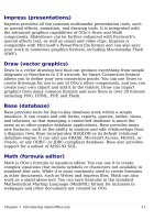
Figure 105 shows some frozen rows and columns. The heavier
horizontal line between rows 3 and 14 and the heavier vertical line
between columns C and H denote the frozen areas Rows 4 through 13
and columns D through G have been scrolled off the page. Because the
first three rows and columns are frozen into place, they remained.
Figure 105. Frozen rows and columns
You can set the freeze point at one row, one column, or both a row and
a column as in Figure 105.
Freezing single rows or columns
1) Click on the header for the row below where you want the freeze
or for the column to the right of where you want the freeze.
2) Select Window > Freeze.
A dark line appears, indicating where the freeze is put.
Freezing a row and a column
1) Click into the cell that is immediately below the row you want
frozen and immediately to the right of the column you want
frozen.
2) Select Window > Freeze.
Two lines appear on the screen, a horizontal line above this cell and a
vertical line to the left of this cell. Now as you scroll around the screen,
everything above and to the left of these lines will remain in view.
142 Getting Started with OpenOffice.org 3

Unfreezing
To unfreeze rows or columns, select Window > Freeze. The check
mark by Freeze will vanish.
Splitting the window
Another way to change the view is by splitting the window—also known
as splitting the screen. The screen can be split either horizontally or
vertically or both. This allows you to have up to four portions of the
spreadsheet in view at any one time.
Why would you want to do this? Imagine you have a large spreadsheet
and one of the cells has a number in it which is used by three formulas
in other cells. Using the split screen technique, you can position the
cell containing the number in one section and each of the cells with
formulas in the other sections. Then you can change the number in the
cell and watch how it affects each of the formulas.
Figure 106. Split screen example
Splitting the screen horizontally
To split the screen horizontally:
1) Move the mouse pointer into the vertical scroll bar, on the right-
hand side of the screen, and place it over the small button at the
top with the black triangle.
Figure 107. Split screen bar on vertical scroll bar
Chapter 5 Getting Started with Calc 143
Split screen bar
2) Immediately above this button you will see a thick black line
(Figure 107). Move the mouse pointer over this line and it turns
into a line with two arrows (Figure 108).
Figure 108. Split screen bar on
vertical scroll bar with cursor
3) Hold down the left mouse button and a gray line appears, running
across the page. Drag the mouse downwards and this line follows.

4) Release the mouse button and the screen splits into two views,
each with its own vertical scroll bar.
Notice in Figure 106, the ‘Beta’ and the ‘A0’ values are in the upper
part of the window and other calculations are in the lower part. You
may scroll the upper and lower parts independently. Thus you can
make changes to the Beta and A0 values and watch their affects on the
calculations in the lower half of the window.
You can also split the window vertically as described below—with the
same results, being able to scroll both parts of the window
independently. With both horizontal and vertical splits, you have four
independent windows to scroll.
Splitting the screen vertically
To split the screen vertically:
1) Move the mouse pointer into the horizontal scroll bar at the
bottom of the screen and place it over the small button on the
right with the black triangle.
Figure 109: Split bar on horizontal scroll bar
2) Immediately to the right of this button is a thick black line (Figure
109). Move the mouse pointer over this line and it turns into a
line with two arrows.
144 Getting Started with OpenOffice.org 3
Split screen bar
3) Hold down the left mouse button and a gray line appears, running
up the page. Drag the mouse to the left and this line follows.
4) Release the mouse button and the screen is split into two views,
each with its own horizontal scroll bar.
Note
Splitting the screen horizontally and vertically at the same
time gives four views, each with its own vertical and
horizontal scroll bars.

Removing split views
To remove a split view, do any of the following:
• Double-click on each split line.
• Click on and drag the split lines back to their places at the ends of
the scroll bars.
• Select Window > Split to remove all split lines at the same time.
Tip
You can also split the screen using a menu command. Click in a
cell that is immediately below and immediately to the right of
where you wish the screen to be split, and choose Window >
Split.
Entering data using the keyboard
Most data entry in Calc can be accomplished using the keyboard.
Entering numbers
Click in the cell and type in the number using the number keys on
either the main keyboard or the numeric keypad.
To enter a negative number, either type a minus (–) sign in front of it or
enclose it in parentheses (brackets), like this: (1234).
By default, numbers are right-aligned and negative numbers have a
leading minus symbol.
Entering text
Click in the cell and type the text. Text is left-aligned by default.
Chapter 5 Getting Started with Calc 145
Entering numbers as text
If a number is entered in the format
01481
, Calc will drop the leading
0. (Exception: see Tip below.) To preserve the leading zero, for example
for telephone area codes, type an apostrophe before the number, like
this: '01481.

The data is now regarded as text by Calc. Formulas and functions will
treat the entry like any other text entry, which typically results in it
being a zero in a formula, and being ignored in a function.
Tip
Numbers can have leading zeros and be regarded as numbers
(as opposed to text) if the cell is formated appropriately. Right-
click on the cell and chose Format Cells > Numbers. Adjust
the leading zeros setting to add leading zeros to numbers.
Note
When using an apostrophe to allow a leading 0 to be displayed,
the apostrophe is not visible in the cell after the
Enter
key is
pressed—
if
the apostrophe is a plain apostrophe (not a “smart
quote” apostrophe). If “smart quotes” are selected for
apostrophes, the apostrophe remains visible in the cell.
To choose the type of apostrophe, use Tools > AutoCorrect >
Custom Quotes. The selection of the apostrophe type affects
both Calc and Writer.
Caution
When a number is formatted as text care must be taken that
the cell containing the number is not used in a formula since
Calc will ignore the value.
Entering dates and times
Select the cell and type the date or time. You can separate the date
elements with a slant (/) or a hyphen (–) or use text such as 10 Oct 03.
Calc recognizes a variety of date formats. You can separate time
elements with colons such as 10:43:45.

Speeding up data entry
Entering data into a spreadsheet can be very labor-intensive, but Calc
provides several tools for removing some of the drudgery from input.
The most basic ability is to drop and drag the contents of one cell to
another with a mouse. However, Calc also includes several other tools
for automating input, especially of repetitive material. They include the
146 Getting Started with OpenOffice.org 3
Fill tool, selection lists, and the ability to input information into
multiple sheets of the same document.
Using the Fill tool on cells
At its simplest, the Fill tool is a way to duplicate existing content. Start
by selecting the cell to copy, then drag the mouse in any direction (or
hold down the Shift key and click in the last cell you want to fill), and
then choose Edit > Fill and the direction in which you want to copy:
Up, Down, Left or Right.
Caution
Choices that are not available are grayed out, but you can still
choose the opposite direction from what you intend, which
could cause you to overwrite cells accidentally unless you are
careful.
Tip
A shortcut way to fill cells is to grab the “handle” in the lower
right-hand corner of the cell and drag it in the direction you
want to fill.
Figure 110: Using the Fill tool
You can also use the fill tool selecting some existing series of data that
you want to extend. If the interval between the values in the selected
cells is constant, Calc will try to guess and fill the selection with values
that continue the sequence. For example, if you select three cells
containing the values 1, 2 and 3 and fill the subsequent cell Calc will

insert the value 4.
Using a fill series
A more complex use of the Fill tool is to use a fill series. The default
lists are for the full and abbreviated days of the week and the months
of the year, but you can create your own lists as well.
Chapter 5 Getting Started with Calc 147
To add a fill series to a spreadsheet, select the cells to fill, choose Edit
> Fill > Series. In the Fill Series dialog, select AutoFill as the
Series
type
, and enter as the
Start value
an item from any defined series. The
selected cells then fill in the other items on the list sequentially,
repeating from the top of the list when they reach the end of the list.
Figure 111: Specifying the start of a fill series (result is in Figure 112)
You can also use Edit > Fill > Series
to create a one-time fill series for
numbers by entering the start and end
values and the increment. For example,
if you entered start and end values of 1
and 7 with an increment of 2, you would
get the sequence of 1, 3, 5, 7.
In all these cases, the Fill tool creates
only a momentary connection between
the cells. Once they are filled, the cells
have no further connection with one
another.
Defining a fill series
To define a fill series, go to Tools > Options > OpenOffice.org Calc

> Sort Lists. This dialog shows the previously-defined series in the
Lists
box on the left, and the contents of the highlighted list in the
Entries
box.
148 Getting Started with OpenOffice.org 3
Figure 112: Result of fill series
selection shown in Figure 111
Figure 113: Predefined fill series
Click New. The
Entries
box is cleared. Type the series for the new list
in the
Entries
box (one entry per line), and then click Add.
Figure 114: Defining a new fill series
Using selection lists
Selection lists are available only for text, and are
limited to using only text that has already been entered
in the same column.
To use a selection list, select a blank cell and press
Ctrl+D
. A drop-down list appears of any cell in the same
column that either has at least one text character or
whose format is defined as Text. Click on the entry you
require.
Sharing content between sheets
You might want to enter the same information in the same cell on
multiple sheets, for example to set up standard listings for a group of
individuals or organizations. Instead of entering the list on each sheet

individually, you can enter it in all the sheets at once. To do this, select
all the sheets, then enter the information in the current one.
Chapter 5 Getting Started with Calc 149
Caution
This technique overwrites any information that is already in
the cells on the other sheets—without any warning. For this
reason, when you are finished, be sure to deselect all the tabs,
so that each sheet can be edited without affecting any others.
Editing data
Editing data is done is in much the same way as it is entered. The first
step is selecting the cell containing the data to be edited.
Removing data from a cell
Data can be removed (deleted) from a cell in several ways.
Removing data only
The data alone can be removed from a cell without removing any of the
formatting of the cell. Click in the cell to select it, and then press the
Backspace
key.
Removing data and formatting
The data and the formatting can be removed from a cell at the same
time. Press the
Delete
key (or right-click and choose Delete Contents,
or use Edit > Delete Contents) to open the Delete Contents dialog
(Figure 115). From this dialog, the different aspects of the cell can be
deleted. To delete everything in a cell (contents and format), check
Delete all.
Figure 115: Delete Contents dialog
150 Getting Started with OpenOffice.org 3