Quantitative Methods for Business chapter 7 potx

CHAPTER
Two-way traffic –
summarizing and
representing relationships
between two variables
7
Chapter objectives
This chapter will help you to:
■ explore links between quantitative variables using bivariate
analysis
■ measure association between quantitative variables using
Pearson’s product moment correlation coefficient and the
coefficient of determination
■ quantify association in ordinal data using Spearman’s rank
correlation coefficient
■ represent the connection between two quantitative variables
using simple linear regression analysis
■ use the technology: correlation and regression in EXCEL,
MINITAB and SPSS
■ become acquainted with business uses of correlation and
regression
224 Quantitative methods for business Chapter 7
This chapter is about techniques that you can use to study relation-
ships between two variables. The types of data set that these techniques
are intended to analyse are called bivariate because they consist of
observed values of two variables. The techniques themselves are part of
what is known as bivariate analysis.
Bivariate analysis is of great importance to business. The results of
this sort of analysis have affected many aspects of business consider-
ably. The establishment of the relationship between smoking and
health problems transformed the tobacco industry. The analysis of sur-

vival rates of micro-organisms and temperature is crucial to the setting
of appropriate refrigeration levels by food retailers. Marketing strate-
gies of many organizations are often based on the analysis of consumer
expenditure in relation to age or income.
The chapter will introduce you to some of the techniques that com-
panies and other organizations use to analyse bivariate data. The tech-
niques you will meet here are correlation analysis and regression analysis.
Suppose you have a set of bivariate data that consist of observations
of one variable, X, and the associated observations of another variable,
Y, and you want to see if X and Y are related. For instance, the Y vari-
able could be sales of ice cream per day and the X variable the daily
temperature, and you want to investigate the connection between tem-
perature and ice cream sales. In such a case correlation analysis
enables us to assess whether there is a connection between the two vari-
ables and, if so, how strong that connection is.
If correlation analysis tells us there is a connection we can use regres-
sion analysis to identify the exact form of the relationship. It is essential
to know this if you want to use the relationship to make predictions, for
instance if we want to predict the demand for ice cream when the daily
temperature is at a particular level.
The assumption that underpins bivariate analysis is that one variable
depends on the other. The letter Y is used to represent the dependent
variable, the one whose values are believed to depend on the other
variable. This other variable, represented by the letter X, is called the
independent variable. The Y or dependent variable is sometimes known
as the response because it is believed to respond to changes in the value
of the X variable. The X variable is also known as the predictor because
it might help us to predict the values of Y.
7.1 Correlation analysis
Correlation analysis is a way of investigating whether two variables are cor-

related, or connected with each other. We can study this to some extent
by using a scatter diagram to portray the data, but such a diagram can
only give us a visual ‘feel’ for the association between two variables, it
doesn’t actually measure the strength of the connection. So, although a
scatter diagram is the thing you should begin with to carry out bivariate
analysis, you need to calculate a correlation coefficient if you want a precise
way of assessing how closely the variables are related.
In this section we shall consider two correlation coefficients. The
first and more important is Pearson’s product moment correlation coef-
ficient, related to which is the coefficient of determination. The sec-
ond is Spearman’s rank correlation coefficient. Pearson’s coefficient is
suitable for assessing the strength of the connection between quantita-
tive variables, variables whose values are interval or ratio data (you may
find it helpful to refer back to section 4.3 of Chapter 4 for more on
types of data). Spearman’s coefficient is designed for variables whose
values are ranked, and is used to assess the connection between two
variables, one or both of which have ordinal values.
7.1.1 Pearson’s product moment correlation coefficient
Pearson’s correlation coefficient is similar to the standard deviation in
that it is based on the idea of dispersion or spread. The comparison is
not complete because bivariate data are spread out in two dimensions;
if you look at a scatter diagram you will see that the points representing
the data are scattered both vertically and horizontally.
The letter r is used to represent the Pearson correlation coefficient
for sample data. Its Greek counterpart, the letter ␳ (‘rho’) is used to
represent the Pearson correlation coefficient for population data. As is
the case with other summary measures, it is very unlikely that you will
have to find the value of a population correlation coefficient because of
the cost and practical difficulty of studying entire populations.
Pearson’s correlation coefficient is a ratio; it compares the co-ordinated

scatter to the total scatter. The co-ordinated scatter is the extent to
which the observed values of one variable, X, vary in co-ordination
with, or ‘in step with’ the observed values of a second variable, Y. We
use the covariance of the values of X and Y, Cov
XY
to measure the degree
of co-ordinated scatter.
To calculate the covariance you have to multiply the amount that
each x deviates from the mean of the X values, x
_
, by the amount that its
corresponding y deviates from the mean of the Y values, y
_
. That is, for
every pair of x and y observations you calculate:
()()xxyy ϪϪ
Chapter 7 Two-way traffic – relationships between two variables 225
The result will be positive whenever the x and y values are both bigger
than their means, because we will be multiplying two positive deviations
together. It will also be positive if both the x and y values are smaller
than their means, because both deviations will be negative and the
result of multiplying them together will be positive. The result will only
be negative if one of the deviations is positive and the other negative.
The covariance is the total of the products from this process divided
by n, the number of pairs of observations, minus one. We have to
divide by n Ϫ 1 because the use of the means in arriving at the devi-
ations results in the loss of a degree of freedom.
The covariance is positive if values of X below x
_
tend to be associated

with values of Y below y
_
, and values of X above x
_
tend to be associated
with values of Y above y
_
. In other words if high x values occur with high
y values and low x values occur with low y values we will have a positive
covariance. This suggests that there is a positive or direct relationship
between X and Y, that is, if X goes up we would expect Y to go up as
well, and vice versa. If you compared the income of a sample of con-
sumers with their expenditure on clothing you would expect to find a
positive relationship.
The covariance is negative if values of X below x
_
are associated with
values of Y above y
_
, and vice versa. The low values of X occur with the
high values of Y, and the high values of X occur with the low values of Y.
This is a negative or inverse relationship. If you compared the prices of
articles of clothing with demand for them, economic theory suggests
you might expect to find an inverse relationship.
Cov
( )
1
XY
xxyy
n

ϭ
ϪϪ
Ϫ
()
()
∑
226 Quantitative methods for business Chapter 7
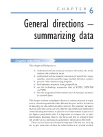
Example 7.1
Courtka Clothing sells six brands of shower-proof jacket. The prices and the numbers
sold in a week are:
Plot a scatter diagram and calculate the covariance.
In Figure 7.1 number sold has been plotted on the Y, or vertical, axis and price has
been plotted on the X, or horizontal, axis. We are assuming that number sold depends
on price rather than the other way round.
Price 18 20 25 27 28 32
Number sold 8 6 5 2 2 1
The other input we need to obtain a Pearson correlation coefficient is
some measure of total scatter, some way of assessing the horizontal and
vertical dispersion. We do this by taking the standard deviation of the
x values, which measures the horizontal spread, and multiplying by the
standard deviation of the y values, which measures the vertical spread.
Chapter 7 Two-way traffic – relationships between two variables 227
To calculate the covariance we need to calculate deviations from the mean for every
x and y value.
x
_
ϭ (18 ϩ 20 ϩ 25 ϩ 27 ϩ 28 ϩ 32)/6 ϭ 150/5 ϭ 25
y
_
ϭ (8 ϩ 6 ϩ 5 ϩ 2 ϩ 2 ϩ 1)/6 ϭ 24/6 ϭ 4

Covariance ϭ ∑(x Ϫ x
_
)(y Ϫ y
_
)/(n Ϫ 1) ϭϪ69/5 ϭϪ13.8
352515
10
9
8
7
6
5
4
3
2
1
0
Price (£)
Number sold
Figure 7.1
Prices of jackets and numbers sold
Numbers
Price (x) x
_
(x Ϫ x
_
) sold (y) y
_
(y Ϫ y
_

)(x Ϫ x
_
)(y Ϫ y
_
)
18 25 Ϫ7844 Ϫ28
20 25 Ϫ5642 Ϫ10
25 25 0 5 4 1 0
27 25 2 2 4 Ϫ2 Ϫ4
28 25 3 2 4 Ϫ2 Ϫ6
32 25 7 1 4 Ϫ3 Ϫ21
∑(x Ϫ x
_
)(y Ϫ y
_
) ϭϪ69
The Pearson correlation coefficient, r, is the covariance of the x and
y values divided by the product of the two standard deviations.
There are two important things you should note about r:
■ It can be either positive or negative because the covariance
can be negative or positive.
■ It cannot be larger than 1 or Ϫ1 because the co-ordinated scat-
ter, measured by the covariance, cannot be larger than the total
scatter, measured by the product of the standard deviations.
A more direct approach to calculating the value of the Pearson cor-
relation coefficient is to use the following formula, which is derived
from the approach we used in Examples 7.1 and 7.2:
r
nxy x y
nx x ny y

*
*
22
ϭ
Ϫ
ϪϪ
∑∑∑
(
)
∑∑
(
)
(
)
∑∑
(
)
(
)
22
r
ss
XY
xy

Cov
( * )
ϭ
228 Quantitative methods for business Chapter 7
Example 7.2

Calculate the correlation coefficient for the data in Example 7.1.
We need to calculate the sample standard deviation for X and Y.
From Example 7.1: Covariance ϭϪ13.8
Sample standard deviation of X:
Sample standard deviation of Y:
Correlation coefficient: r ϭ (Ϫ13.8)/(5.215 * 2.757)
ϭϪ13.8/14.41 ϭϪ0.960
syyn
y
1 38/5 2.757ϭϪ Ϫϭ ϭ∑()/()
2
sxxn
x
1 136/5 5.215ϭϪ Ϫϭ ϭ∑()/()
2
Number
Price (x) x
_
(x Ϫ x
_
)(x Ϫ x
_
)
2
sold (y) y
_
(y Ϫ y
_
)(y Ϫ y
_

)
18 25 Ϫ749 84416
20 25 Ϫ525 6424
25 25 0 0 5 4 1 1
27 25 2 4 2 4 Ϫ24
28 25 3 9 2 4 Ϫ24
32 25 7 49 1 4 Ϫ39
136 38
The advantage of this approach is that there are no subtractions
between the observations and their means as it involves simply adding
up the observations and their squares.
Chapter 7 Two-way traffic – relationships between two variables 229
Example 7.3
Calculate the Pearson correlation coefficient for the data in Example 7.1 without sub-
tracting observations from means.
r
6 * 531 150 * 24
* 3886 150 * 6 * 134 24
3186 3600
22500 * (804 576)
414
816 * 228
414
186048
414
0.960
22
ϭ
Ϫ
ϪϪ

ϭ
Ϫ
ϪϪ
ϭ
Ϫ
ϭ
Ϫ
ϭ
Ϫ
ϭϪ
6
23316
431 333
(
)
(
)
()
.
Number
Price (x) x
2
sold (y) y
2
xy
18 324 8 64 144
20 400 6 36 120
25 625 5 25 125
27 729 2 4 54
28 784 2 4 56

32 1024 1 1 32
∑x ϭ 150 ∑x
2
ϭ 3886 ∑y ϭ 24 ∑y
2
ϭ 134 ∑xy ϭ 531 n ϭ 6
As you can see, calculating a correlation coefficient, even for a fairly
simple set of data, is quite laborious. In practice Pearson correlation
coefficients are seldom calculated in this way because many calculators
and just about all spreadsheet and statistical packages have functions
to produce them. Try looking for two-variable functions on your calcu-
lator and refer to section 7.3 later in this chapter for guidance on soft-
ware facilities.
What should we conclude from the analysis of the data in Example
7.1? Figure 7.1 shows that the scatter of points representing the data
nearly forms a straight line, in other words, there is a pronounced linear
pattern. The diagram also shows that this linear pattern goes from the
top left of the diagram to the bottom right, suggesting that fewer of the
more expensive garments are sold. This means there is an inverse rela-
tionship between the numbers sold and price.
What does the Pearson correlation coefficient in Example 7.2 tell us?
The fact that it is negative, Ϫ0.96, confirms that the relationship between
the numbers sold and price is indeed an inverse one. The fact that it is
very close to the maximum possible negative value that a Pearson
correlation coefficient can take, Ϫ1, indicates that there is a strong
association between the variables.
The Pearson correlation coefficient measures linear correlation, the
extent to which there is a straight-line relationship between the vari-
ables. Every coefficient will lie somewhere on the scale of possible val-
ues, that is between Ϫ1 and ϩ1 inclusive.

A Pearson correlation coefficient of ϩ1 tells us that there is a perfect
positive linear association or perfect positive correlation between the vari-
ables. If we plotted a scatter diagram of data that has such a relation-
ship we would expect to find all the points lying in the form of an
upward-sloping straight line. You can see this sort of pattern in Figure 7.2.
A correlation coefficient of Ϫ1 means we have perfect negative correl-
ation, which is illustrated in Figure 7.3.
In practice you are unlikely to come across a Pearson correlation coef-
ficient of precisely ϩ1 or Ϫ1, but you may well meet coefficients that are
positive and fairly close to ϩ1 or negative and fairly close to Ϫ1. Such
values reflect good positive and good negative correlation respectively.
230 Quantitative methods for business Chapter 7
Figure 7.2
Perfect positive
correlation
6543210
20
10
0
X
Y
Figure 7.4 shows a set of data with a correlation coefficient of ϩ0.9.
You can see that although the points do not form a perfect straight line
they form a pattern that is clearly linear and upward sloping.
Figure 7.5 portrays bivariate data that has a Pearson correlation coef-
ficient of Ϫ0.9. The points do not lie in a perfect straight downward
line but you can see a clear downward linear pattern.
The closer your Pearson correlation coefficient is to ϩ1 the better the
positive correlation. The closer it is to Ϫ1 the better the negative cor-
relation. It follows that the nearer the coefficient is to zero the weaker

Chapter 7 Two-way traffic – relationships between two variables 231
Figure 7.3
Perfect negative
correlation
6543210
20
10
0
X
Y
Figure 7.4
Good positive
correlation
6543210
20
10
0
X
Y
the connection between the two variables. Figure 7.6 shows a sample of
observations of two variables with a coefficient close to zero, which pro-
vides little evidence of any correlation.
It is important to bear in mind that the Pearson correlation coefficient
assesses the strength of linear relationships between two variables. It is
quite possible to find a low or even zero correlation coefficient where
the scatter diagram shows a strong connection. This happens when the
relationship between the two variables is not linear.
232 Quantitative methods for business Chapter 7
Figure 7.5
Good negative

correlation
6543210
20
10
0
X
Y
Figure 7.6
Zero correlation
6543210
20
10
0
X
Y
Figure 7.7 shows that a clear non-linear relationship exists between
the variables yet the Pearson correlation coefficient for the data it por-
trays is zero.
If you have to write about correlation analysis results you may find
the following descriptions useful:
The things to remember about the sample Pearson correlation coef-
ficient, r, are:
■ It measures the strength of the connection or association
between observed values of two variables.
■ It can take any value from Ϫ1 to ϩ1 inclusive.
■ If it is positive it means there is a direct or upward-sloping
relationship.
■ If it is negative it means there is an inverse or downward-sloping
relationship.
Chapter 7 Two-way traffic – relationships between two variables 233

Figure 7.7
A non-linear
relationship
6543210
20
10
0
X
Y
Values of r Suitable adjectives
ϩ0.9 to ϩ1.0 Strong, positive
ϩ0.6 to ϩ0.89 Fair/moderate, positive
ϩ0.3 to ϩ0.59 Weak, positive
0.0 to ϩ0.29 Negligible/scant positive
0.0 to Ϫ0.29 Negligible/scant negative
Ϫ0.3 to Ϫ0.59 Weak, negative
Ϫ0.6 to Ϫ0.89 Fair/moderate, negative
Ϫ0.9 to Ϫ1.0 Strong, negative
■ The further it is from zero the stronger the association.
■ It only measures the strength of linear relationships.
At this point you may find it useful to try Review Questions 7.1 to 7.5
at the end of the chapter.
7.1.2 The coefficient of determination
The square of the Pearson correlation coefficient is also used as a way of
measuring the connection between variables. Although it is the square
of r, the upper case is used in representing it, R
2
. It is called the coeffi-
cient of determination because it can help you to assess how much the
values of one variable are decided or determined by the values of another.

As we saw, the Pearson correlation coefficient is based on the stand-
ard deviation. Similarly the square of the correlation coefficient is
based on the square of the standard deviation, the variance.
Like the correlation coefficient, the coefficient of determination is a
ratio, the ratio of the amount of the variance that can be explained by
the relationship between the variables to the total variance in the data.
Because it is a ratio it cannot exceed one and because it is a square it is
always a positive value. Conventionally it is expressed as a percentage.
You may find R
2
an easier way to communicate the strength of the rela-
tionship between two variables. Its only disadvantage compared to the
correlation coefficient is that the figure itself does not convey whether
the association is positive or negative. However, there are other ways of
showing this, including the scatter diagram.
7.1.3 Spearman’s rank correlation coefficient
If you want to investigate links involving ordinal or ranked data you
should not use the Pearson correlation coefficient as it is based on the
234 Quantitative methods for business Chapter 7
Example 7.4
Calculate the coefficient of determination, R
2
, for the data in Example 7.1.
In Example 7.2 we calculated that the Pearson correlation coefficient for these data
was Ϫ0.960. The square of Ϫ0.960 is 0.922 or 92.2%. This is the value of R
2
. It means
that 92.2% of the variation in the numbers of jackets sold can be explained by the vari-
ation in the prices.
arithmetic measures of location and spread, the mean and the stand-

ard deviation. Fortunately there is an alternative, the Spearman rank
correlation coefficient.
It is possible to use the Spearman coefficient with interval and ratio
data provided the data are ranked. You find the value of the coefficient
from the ranked data rather than the original observations you would
use to get the Pearson coefficient. This may be a preferable alternative
as you may find calculating the Spearman coefficient easier. If your
original observations contain extreme values the Pearson coefficient
may be distorted by them, just as the mean is sensitive to extreme values,
in which case the Spearman coefficient may be more reliable.
To calculate the Spearman coefficient, usually represented by the
symbol r
s
, subtract the ranks of your y values from the ranks of their
corresponding x values to give a difference in rank, d, for each pair of
observations. Next square the differences and add them up to get ∑d
2
.
Multiply the sum of the squared differences by 6 then divide the result
by n, the number of pairs of observations, multiplied by the square of
n minus one. Finally subtract the result from one to arrive at the coef-
ficient. The procedure can be expressed as follows:
r
d
nn
s
1
6
1
ϭϪ

Ϫ
∑
(
)
2
2
Chapter 7 Two-way traffic – relationships between two variables 235
Example 7.5
The total annual cost of players’ wages for eight football clubs and their final league
positions are as follows:
Work out the Spearman coefficient for the correlation between the league positions
and wages bills of these clubs.
Wages bill (£m) Final league position
45 1
32 2
41 3
13 4
27 5
15 6
18 7
22 8
The interpretation of the Spearman coefficient is the same as we use
for the Pearson coefficient. In Example 7.5 the coefficient is positive,
indicating positive correlation and rather less than ϩ1 suggesting the
degree of correlation is modest.
Using the Spearman coefficient with ranked data that contains ties is
not quite as straightforward. The ranks for the tied elements need to
be adjusted so that they share the ranks they would have had if they
were not equal. For instance if two elements are ranked second equal
in effect they share the second and third positions. To reflect this we

would give them a rank of 2.5 each.
236 Quantitative methods for business Chapter 7
One variable, league position, is already ranked, but before we can calculate the coef-
ficient we have to rank the values of the other variable, the wage bill.
r
s
2
1
6 * 30
8(8 1)
1
180
8(64 1)
1
180
8 * 63
1
180
504
1 0.357 0.643
ϭϪ
Ϫ
ϭϪ
Ϫ
ϭϪ
ϭϪ ϭϪ ϭ
Rank of wages bill League position dd
2
1100
32ϩ11

23ϩ11
84ϩ416
45Ϫ11
76ϩ11
67Ϫ11
58Ϫ39
∑d
2
ϭ 30 n ϭ 8
Example 7.6
Rank the data in Example 7.1 from lowest to highest and find the Spearman rank cor-
relation coefficient for the prices of the jackets and the number of jackets sold.
Price (x) Rank (x) Number sold (y) Rank (y) dd
2
18 1 8 6 1 Ϫ 6 ϭϪ525
20 2 6 5 2 Ϫ 5 ϭϪ39
(Continued)
Chapter 7 Two-way traffic – relationships between two variables 237
r
s
2
1
6 * 68.5
6(6 1)
1
411
6(36 1)
1
411
6 * 35

1
411
210
1 1.957 0.957
ϭϪ
Ϫ
ϭϪ
Ϫ
ϭϪ
ϭϪ ϭϪ ϭϪ
In Example 7.6 the Spearman coefficient for the ranked data is very
similar to the value of the Pearson coefficient we obtained in Example
7.2 for the original observations – 0.960. Both results show that the cor-
relation between prices and sales is strong and negative.
At this point you may find it useful to try Review Questions 7.6 to 7.9
at the end of the chapter.
7.2 Simple linear regression analysis
Measuring correlation tells you how strong the linear relationship
between two variables might be but it doesn’t tell us exactly what that
relationship is. If we need to know about the way in which two variables
are related we have to use the other part of basic bivariate analysis,
regression analysis.
The simplest form of this technique, simple linear regression (which is
often abbreviated to SLR), enables us to find the straight line most
appropriate for representing the connection between two sets of
observed values. Because the line that we ‘fit’ to our data can be used
to represent the relationship it is rather like an average in two dimen-
sions, it summarizes the link between the variables.
Simple linear regression is called simple because it analyses two vari-
ables, it is called linear because it is about finding a straight line, but

why is it called regression, which actually means going backwards? The
answer is that the technique was first developed by the nineteenth cen-
tury scientist Sir Francis Galton, who wanted a way of representing how
Price (x) Rank (x) Number sold (y) Rank (y) dd
2
25 3 5 4 3 Ϫ 4 ϭϪ11
27 4 2 2.5 4 Ϫ 2.5 ϭ 1.5 2.25
28 5 2 2.5 5 Ϫ 2.5 ϭ 2.5 6.25
32 6 1 1 6 Ϫ 1 ϭ 525
∑d
2
ϭ 68.5 n ϭ 6
the heights of children were genetically constrained or ‘regressed’ by
the heights of their parents.
In later work you may encounter multiple regression, which is used to
analyse relationships between more than two variables, and non-linear
regression, which is used to analyse relationships that do not have a
straight-line pattern.
You might ask why it is necessary to have a technique to fit a line to a
set of data? It would be quite easy to look at a scatter diagram like
Figure 7.1, lay a ruler close to the points and draw a line to represent
the relationship between the variables. This is known as fitting a line
‘by eye’ and is a perfectly acceptable way of getting a quick approxi-
mation, particularly in a case like Figure 7.1 where there are few points
which form a clear linear pattern.
The trouble with fitting a line by eye is that it is inconsistent and
unreliable. It is inconsistent because the position of the line depends
on the judgement of the person drawing the line. Different people will
produce different lines for the same data.
For any set of bivariate data there is one line that is the most appro-

priate, the so-called ‘best-fit’ line. There is no guarantee that fitting a line
by eye will produce the best-fit line, so fitting a line by eye is unreliable.
We need a reliable, consistent way of finding the line that best fits a
set of plotted points, which is what simple linear regression analysis is.
It is a technique that finds the line of best-fit, the line that travels as
closely as possible to the plotted points. It identifies the two defining
characteristics of that line, its intercept, or starting point, and its slope, or
rate of increase or decrease. These are illustrated in Figure 7.8.
We can use these defining characteristics to compose the equation
of the line of best fit, which represents the line using symbols. The
equation enables us to plot the line itself.
Simple linear regression is based on the idea of minimizing the dif-
ferences between a line and the points it is intended to represent. Since
238 Quantitative methods for business Chapter 7
Figure 7.8
The intercept and
slope of a line
Slope (b)
Intercept (a)
all the points matter, it is the sum of these differences that needs to be
minimized. In other words, the best-fit line is the line that results in a
lower sum of differences than any other line would for that set of data.
The task for simple linear regression is a little more complicated
because the difference between a point and the line is positive if the
point is above the line, and negative if the point is below the line. If we
were to add up these differences we would find that the negative and
positive differences cancel each other out.
This means the sum of the differences is not a reliable way of judg-
ing how well a line fits a set of points. To get around this problem, sim-
ple linear regression is based on the squares of the differences because

they will always be positive.
The best-fit line that simple linear regression finds for us is the line
which takes the path that results in there being the least possible sum
Chapter 7 Two-way traffic – relationships between two variables 239
Example 7.7
The amount of profit tax (in £m) paid by three companies in the current financial year
and their respective gross profits (in £m) were:
Which of the two lines best fits the data, the one in Figure 7.9 or the one in Figure 7.10?
The deviations between the points and the line in Figure 7.9 (y ϭϪ3.5 ϩ 0.4x) are,
from left to right, ϩ1.5, Ϫ1.5 and 0. The total deviation is:
ϩ1.5 ϩ (Ϫ1.5) ϩ 0.0 ϭ 0.0
The deviations between the points and the line in Figure 7.10 (y ϭ 0.2x) are, from left
to right, ϩ1, Ϫ1 and ϩ1. The total deviation is:
ϩ1.0 ϩ (Ϫ1.0) ϩ 1.5 ϭ 1.5
The fact that the total deviation is smaller for Figure 7.9 suggests that its line is the bet-
ter fit. But if we take the sum of the squared deviations the conclusion is different.
Total squared deviation in Figure 7.9
ϭ 1.5
2
ϩ (Ϫ1.5)
2
ϩ 0.0
2
ϭ 2.25 ϩ 2.25 ϩ 0.00 ϭ 4.50
Total squared deviation in Figure 7.10
ϭ 1.0
2
ϩ (Ϫ1.0)
2
ϩ 1.5

2
ϭ 1.00 ϩ 1.00 ϩ 2.25 ϭ 4.25
Profit tax paid (Y) 4.0 3.0 6.5
Gross profit (X) 15.0 20.0 25.0
240 Quantitative methods for business Chapter 7
This apparent contradiction has arisen because the large deviations in Figure 7.9
cancel each other out when we simply add them together.
Figure 7.9
Profit tax and profit
252015
8
7
6
5
4
X
X
X
3
2
1
0
Gross profit (£m)
Profit tax (£m)
Figure 7.10
Profit tax and gross profit
252015
8
7
6

5
4
3
X
X
X
2
1
0
Gross profit (£m)
Profit tax (£m)
of squared differences between the points and the line. For this reason
the technique is sometimes referred to as least squares regression.
For any given set of data, as you can imagine, there are many lines
from which the best-fit line could be chosen. To pick the right one we
could plot each of them in turn and measure the differences using a
ruler. Fortunately, such a laborious procedure is not necessary. Simple
linear regression uses calculus, the area of mathematics that is partly
about finding minimum or maximum values, to find the intercept and
slope of the line of best fit directly from the data.
The procedure involves using two expressions to find, first, the slope
and then the intercept. Since simple linear regression is almost always
used to find the line of best fit from a set of sample data the letters used
to represent the intercept and the slope are a and b respectively. The
equivalent Greek letters, ␣ and ␤, are used to represent the intercept
and slope of the population line of best fit.
According to simple linear regression analysis the slope of the line of
best fit:
And the intercept: a ϭ (∑y Ϫ b∑x)/n
These results can then be combined to give the equation of the line of

best fit, which is known as the regression equation:
Y ϭ a ϩ bX
The expressions for getting the slope and intercept of the line of best
fit look daunting, but this need not worry you. If you have to find a
best fit line you can use a statistical or a spreadsheet package, or even a
calculator with a good statistical facility to do the hard work for you.
They are quoted here, and used in Example 7.8 below, merely to show
you how the procedure works.
b
xy x n
xn
( * y)/
(x)
2
ϭ
Ϫ
Ϫ
∑∑∑
∑∑
2
/
Chapter 7 Two-way traffic – relationships between two variables 241
Example 7.8
Find the equation of the line of best fit for the data in Example 7.1 and plot the line.
We need to find four summations: the sum of the x values, the sum of the y values, the
sum of the x squared values and the sum of the products of each pair of x and y values
multiplied together.
Price (x) x
2
Number sold (y) xy

18 324 8 144
20 400 6 120
(Continued)
242 Quantitative methods for business Chapter 7
a ϭ (∑y Ϫ b∑x)/n ϭ (24 Ϫ (Ϫ0.507)150)/6 ϭ (24 ϩ 76.103)/6
ϭ 100.103/6 ϭ 16.684
The equation of the line of best fit is: Y ϭ 16.684 Ϫ 0.507X
Or, in other words, Number sold ϭ 16.684 Ϫ 0.507 Price
b
xy x y n
xn
( * )/
(x)
531 (150 * 24)/6
150 /6
531 3600/6
22500/6
531 600
3750
69
136
0.507
22
ϭ
Ϫ
Ϫ
ϭ
Ϫ
Ϫ
ϭ

Ϫ
Ϫ
ϭ
Ϫ
Ϫ
ϭ
Ϫ
ϭϪ
∑∑∑
∑∑
2
3886
3886 3886
/
Price (x) x
2
Number sold (y) xy
25 625 5 125
27 729 2 54
28 784 2 56
32 1024 1 32
∑x ϭ 150 ∑x
2
ϭ 3886 ∑y ϭ 24 ∑xy ϭ 531
Figure 7.11
The line of best fit for the numbers of jackets sold and their prices
302520
8
7
6

5
4
3
2
1
0
Price (£)
Number sold
Once we have the equation of a regression line we can use its com-
ponents, its intercept and slope, to describe the relationship between
the variables. For instance, the slope of the equation in Example 7.8
suggests that for every £1 increase in the price of a jacket the number
sold will drop by 0.507 jackets, and for every £1 decrease in the price of
a jacket the number sold will increase by 0.507 jackets. Since the slope
is the rate of change in jacket sales with respect to price, the fact that it is
not a whole number is not important.
The intercept of the equation of a regression line is the value that
the Y variable is predicted to take if the X variable has the value zero.
In Example 7.8 the intercept of 16.684 suggests that roughly seventeen
jackets would be ‘sold’ if the price was zero.
You can use a diagram like Figure 7.11 to compare the individual
points of data to the line of best fit. A point below the line indicates that
the y value is relatively low compared to what we would expect given
the x value, for instance in Figure 7.11 the sales of the jacket priced at
£27 are a little lower than we might expect. A point above the line sug-
gests a y value rather greater than we would expect, such as the jacket
priced at £25 in Figure 7.11. Any point far above or below the line
would represent a possible outlier. If, for example, sales of seven jackets
priced at £30 were plotted the point would be far above the line in
Figure 7.11 and would be a possible outlier.

The process of finding a best fit line with regression analysis is a labori-
ous procedure, even with a relatively simple set of data. It is best per-
formed using appropriate computer software or two-variable calculator
functions.
The equation of the line of best fit we derived in Example 7.8 is an
example of a regression ‘model’. It represents how the two variables
are connected based on the sample evidence in Example 7.1. It is the
best linear model that can be found for that set of data.
We can use such an equation to predict values of Y that should occur
with values of X. These are known as expected values of Y because they
are what the line leads us to expect to be associated with the X values.
The symbol yˆ, ‘y-hat’, is used to represent a value of Y that is predicted
using the regression equation, so that we can distinguish it from an
actual y value. That is to say, the regression equation
Y ϭ a ϩ bX
can be used to predict an individual y value that is expected to occur
with an observed x value:
yˆ ϭ a ϩ bx
Chapter 7 Two-way traffic – relationships between two variables 243
244 Quantitative methods for business Chapter 7
7.3 Using the technology: correlation and
regression in EXCEL, MINITAB and SPSS
7.3.1 Excel
For a Pearson correlation coefficient store the observations of your two
variables in adjacent columns of the spreadsheet then
■ Select Data Analysis from the Tools menu.
■ Choose Correlation from the menu in the Data Analysis
command window, click OK and the Correlation window will
appear. The cursor should be in the Input range: box.
■ Click and drag your mouse across the cells in the spreadsheet

that contain your data then click OK.
To produce a regression equation using EXCEL
■ Choose Data Analysis from the Tools pull-down menu and
select Regression from the Data Analysis menu. Click OK.
■ In the Regression window that appears the cursor should be
in the Input Y Range: box.
■ Click and drag your mouse down the column where your y val-
ues are stored then click the Input X Range: box and click and
drag your mouse down the column containing your x values.
Click OK and the output that appear includes the intercept
and slope of the line of best-fit in the Coefficient column
towards the bottom left of the screen. The intercept is in the
first row and the slope is in the second row.
Example 7.9
Use the regression equation from Example 7.8 to find how many jackets priced at £23
Courtka can expect to sell.
The regression equation tells us that: Number sold ϭ 16.684 Ϫ 0.507 Price
If we insert the value ‘23’ where ‘Price’ appears in the equation we can work out what,
according to the equation, the number sold should be.
Number sold (if price is 23) ϭ 16.684 Ϫ 0.507(23)
ϭ 16.684 Ϫ 11.661 ϭ 5.023
This suggests the expected number sold will be 5, as jackets sales must be in whole numbers.
If you would like the line of best fit shown graphically with the scatter
of points representing your data follow the Regression sequence as
above but in the Regression command window look for the Residuals
section towards the bottom and in it click the box to the left of Line Fit
Plots then OK. The graph should appear to the right of the main regres-
sion output. In it the line of best fit is represented as a series of points. To
get a line through these double click on any one of them and the Format
Data Series command window should appear with the Pattern tab dis-

played. Look for the section headed Line to the left of the window and
in it click the button to the left of Automatic then click OK.
7.3.2 MINITAB
You can use MINITAB to produce a correlation coefficient by storing
your x and y values in two columns of the worksheet and selecting Basic
Statistics from the Stat menu. Choose Correlation from the sub-menu
then give the column location of both sets of observations in the com-
mand window and click OK.
For the equation of a line of best fit
■ Select Regression from the Stat menu and choose Regression
from the Regression sub-menu.
■ Specify the column locations of the Response, i.e. the values
of Y, and the Predictor, i.e. the values of X.
■ Click OK and the output that appears has the regression
equation, the equation of the line of best fit, at the top.
If you want a scatter diagram with the line of best fit superimposed
on the scatter, follow the Stat – Regression sequence but choose Fitted
Line Plot from the Regression sub-menu. Specify the column locations
of the Response (Y ): and Predictor (X ): observations in the boxes to
the right of these labels and click OK. The diagram that appears
includes the regression equation and the value of R
2
for the data.
7.3.3 SPSS
To get a correlation coefficient store the values of your two variables in
the worksheet then
■ Choose Correlate from the Analyze pull-down menu and
select Bivariate from the sub-menu.
Chapter 7 Two-way traffic – relationships between two variables 245
246 Quantitative methods for business Chapter 7

■ In the Bivariate Correlations window that appears the loca-
tions of your data are listed on the left.
■ Click the ᭤ symbol to bring them into the Variables: box on
the right.
■ Check that the default setting under Correlation coefficients
is Pearson and click OK.
Note that you can obtain a Spearman coefficient by clicking the button
to the left of Spearman in this part of the window. The results appear
in the output viewer.
For a regression line
■ Choose Regression from the Analyze pull-down menu and
select Linear.
■ In the Linear Regression window click on the column location
of your dependent (Y) variable on the left-hand side then click
the ᭤ symbol to the left of the Dependent box. Click on the
column location of your independent (X) variable then click
the ᭤ symbol to the left of the Independent box then click OK.
■ Look for the table headed Coefficients and the two columns
in it labelled Unstandardized coefficients. In the left-hand
column, headed B, you will find two figures. The upper one,
in the row labelled (Constant), is the intercept of the model
and the lower one is the slope.
If you would like your regression line fitted to the scatter,
■ Obtain a scatter diagram by choosing Scatter from the Graphs
pull-down menu then click the Simple plot type and click
Define.
■ In the Scatterplot window select your Y axis: and X axis: vari-
ables and click OK. The scatter diagram should be in the out-
put viewer.
■ Double left click on it and the Chart 1 – SPSS Chart Editor

window should appear.
■ Click on its Chart pull-down menu and select Options.
■ In the Scatterplot Options window that you should see,
click the button to the left of Total under Fit Line then click
the Fit Options button and click the Linear Regression fit type.
■ Click Continue to get back to the Scatterplot Options window
where you need to click OK.
■ Minimize or delete the Chart 1 – SPSS Chart Editor window
and your scatter plot should now have a line of best fit.
Chapter 7 Two-way traffic – relationships between two variables 247
7.4 Road test: Do they really use
correlation and regression?
In the Kathawala study (1988), 65% of the respondents reported either
moderate, frequent or extensive use of correlation and regression by
their companies, making it one of the most widely used techniques
considered in that survey. They are techniques that you may well
encounter in many business contexts.
In Human Resources Management correlation analysis has been
used to assess the relationship between the performances applicants
achieve in recruitment and selection procedures and how well they
perform as employees following appointment. Simpson (2002) gives
correlation coefficients for a variety of selection methods from inter-
view performance to handwriting. The results suggest that more sys-
tematic approaches like structured interviews are more effective
predictors of job performance than references.
There are laws that prohibit employers from discriminating against
people on the basis of, inter alia, their gender or their ethnicity. Since these
laws were introduced there have been many legal cases based on alleged
discrimination in appointment and promotion procedures. Conway and
Roberts (1986) illustrate how regression analysis has been used in some

of these cases to demonstrate how an individual has not reached the
salary level or grade they might expect given the time they had worked
for their employer. In such models the salary or grade is the dependent
(Y) variable and the length of service is the independent (X) variable.
Health and safety is another area of business in which correlation
and regression is used extensively. In industries where employees are
exposed to hazards the effects on health may well depend on the
extent of exposure to those hazards. This type of analysis is extensively
used in mining. Kuempel et al. (2003) report the results of a recent
study of the relationship between exposure to coal mine dust and lung
disorders in coal miners.
The performance of different sales territories or areas is an import-
ant issue for sales managers in many organizations. It can have a bearing
on, among other things, the allocation of sales staff and commission
levels. Cravens et al. (1972) used regression analysis to examine how a
variety of factors, including the market potential of the sales areas, the
experience of the sales staff working in the areas and the advertising
expenditure in the areas, might influence sales performance in the
areas. They developed a multiple regression model that was able to
predict 72% of the variation in sales territory performance.