Quantitative Methods for Business chapter 8 potx

CHAPTER
Counting the cost –
summarizing money
variables over time
8
Chapter objectives
This chapter will help you to:
■ employ simple and aggregate index numbers to measure price
changes over time
■ work out weighted aggregate price indices: Laspeyre and
Paasche indices
■ adjust figures for the effects of inflation using price indices
■ apply methods of investment appraisal: accounting rate of
return, payback period, net present value, and internal rate of
return
■ use the technology: investment appraisal methods in EXCEL
■ become acquainted with business uses of investment appraisal
In the last two chapters we have looked at ways of summarizing data. In
Chapter 6 we concentrated on measuring the location and spread in uni-
variate (single variable) data, in Chapter 7 we focused on measuring
the strength and direction in bivariate data. In both chapters the data
concerned were cross-sectional data, data relating to the same point or
period of time. In this chapter and the next we will consider ways of sum-
marizing data relating to different periods of time.
256 Quantitative methods for business Chapter 8
Time-based data consist of numerical observations that can be meas-
ured and summarized using the techniques you met in the previous two
chapters. We could, for instance, collect the price of gold at various points
in time and calculate the mean price of gold over the period, or use
correlation analysis to measure the association between the price of gold
and the price of silver at various points in time. However, often the most

important aspect of time-based data is the time factor and the tech-
niques in the previous two chapters would not allow us to bring that out
of the data.
In this chapter we will look at techniques to summarize money variables
that relate to different time periods. We will start by exploring index
numbers and how they can be used to summarize the general movements
in prices over time. Then we will look at how such price indices can be
used to adjust money amounts for the effects of inflation. Later in the
chapter we will consider summarizing amounts of interest accumulated
over time and how this approach is used to assess the worth of investment
projects.
8.1 Index numbers
Data collected over time are very important for the successful perform-
ance of organizations. For instance, such data can reveal trends in con-
sumer expenditure and taste that companies need to follow.
Businesses use information based on data collected by other agencies
over time to help them understand and evaluate the environment in
which they operate. Perhaps the most important and widespread example
of this is the use of index numbers to monitor general trends in prices
and costs. For instance, the Retail Price Index is used as a benchmark
figure in the context of wage bargaining, and Share Price Indices are
reference points in financial decisions companies face.
Most businesses attach a great deal of importance to changes in the
costs of things they buy and the prices of things they sell. During periods
of high inflation these changes are more dramatic; in periods of low
inflation they are modest. Over recent decades, when the level of infla-
tion has fluctuated, companies have had to track general price and cost
movements carefully. To help them do this they use index numbers.
Index numbers can be used to represent movements over time in a
series of single figures. A simple index number is the value of something

at one point in time, maybe the current value, in relation to its value at
another point in time, the base period, multiplied by 100 to give a per-
centage (although the percent sign, %, is not usually written alongside it).
where p
c
represents the price in the current year and p
0
represent the
price in the base year (i.e. period zero).
At this point you may find it useful to try Review Question 8.1 at the
end of the chapter.
Since businesses usually buy and sell more than a single item, a simple
price index is of limited use. Of much greater importance are aggregate
indices that summarize price movements of many items in a single figure.
We can calculate a simple aggregate price index for a combination
of goods by taking the sum of the prices for the goods in the current
period and dividing it by the sum of the prices of the same goods in the
base period. That is
Simple aggregate price index * 100.
c
ϭ
Σ
Σ
p
p
0
Simple price index
current price
base period price
* 100 * 100

c
0
ϭϭ
p
p
Chapter 8 Counting the cost – summarizing money variables over time 257
Example 8.1
Full exhaust systems cost the Remont Repairs garage £156 each in 2003. They cost £125
in 2000. Calculate a simple price index to represent the change in price over the
period.
This tells us that the price of an exhaust system has increased by 24.8% over this period.
Simple price index
current price
base period price
* 100 * 100
156
125
* 100 124.8 to 1 decimal place
c
0
ϭϭ
ϭϭ
p
p
Example 8.2
Remont Repairs regularly buys exhaust systems, car batteries and tyres. The prices of
these goods in 2003 and 2000 are given in the following table.
Calculate a simple aggregate price index to compare the prices in 2003 to the prices
in 2000.
At this point you may find it useful to try Review Questions 8.2 and 8.3

at the end of the chapter.
The result we obtained in Example 8.2 may well be more useful
because it is an overall figure that includes all the commodities. However,
it does not differentiate between prices of items that may be purchased
in greater quantity than other items, which implies that their prices are
of much greater significance than prices of less important items.
In a simple aggregate price index each price is given equal prom-
inence, you can see that it appears once in the expression. Its numerical
‘clout’ depends simply on whether it is a large or small price. In Example
8.2, the result, 125.3, is close to the value of the simple price index of
the exhaust system calculated in Example 8.1, 124.8. This is because
the exhaust system happens to have the largest price in the set.
In practice, the importance of the price of an item is a reflection of the
quantity that is bought as well as the price itself. To measure changes in
movements of prices in a more realistic way we need to weight each
price in proportion to the quantity purchased and calculate a weighted
aggregate price index.
There are two ways we can do this. The first is to use the quantity figure
from the base year, represented by the symbol q
0
, to weight the price of
each item. This type of index is known as the Laspeyre price index. To
calculate it we need to work out the total cost of the base period quan-
tities at current prices, divide that by the total cost of the base period
quantities at base period prices, and multiply the result by 100:
Laspeyre price index * 100
0c
ϭ
Σ
Σ

qp
qp
00
258 Quantitative methods for business Chapter 8
Simple aggregate price index:
This result indicates that prices paid by the garage increased by 25.3% from 2000 to
2003.
Σ
Σ
p
p
c
* 100
156 35 32
25 28
* 100
223
178
* 100 125.3 to 1 decimal place
0
125
ϭ
ϩϩ
ϩϩ
ϭϭ
2000 2003
Exhaust system £125 £156
Battery £25 £35
Tyre £28 £32
The Laspeyre technique uses quantities that are historical. The advantage

of this is that such figures are usually readily available. The disadvantage
is that they may not accurately reflect the quantities used in the current
period.
The alternative approach, which is more useful when quantities used
have changed considerably, is to use quantity figures from the current
period, q
c
. This type of index is known as the Paasche price index. To
calculate it you work out the total cost of the current period quantities
at current prices, divide that by the total cost of the current period
quantities at base period prices, and multiply the result by 100:
Paasche price index * 100
cc
c
ϭ
Σ
Σ
qp
qp
0
Chapter 8 Counting the cost – summarizing money variables over time 259
Example 8.3
The garage records show that in 2000 50 exhaust systems, 400 batteries and 1000 tyres
were purchased. Use these figures and the price figures from Example 8.2 to produce a
Laspeyre price index to compare the prices of 2003 to those of 2000.
This suggests that the prices have increased by 21.6% between 2000 and 2003.
The result is lower than the figure obtained in Example 8.2, 125.3, because the exhaust
system price has the lowest weighting and tyres, which have the lowest price change,
have the highest weighting.
Σ

Σ
qp
qp
0c
*
100
(50
*
156) (400
*
35) (1000
*
32)
*
125 (400
*
25) (1000
*
28)
*
100
53800
44250
*
100
121.6 to 1 decimal place
00
50
ϭ
ϩϩ

ϩϩ
ϭ
ϭ
()
Example 8.4
In 2003 the garage purchased 50 exhaust systems, 600 batteries and 750 tyres. Use these
figures and the price figures from Example 8.2 to produce a Paasche price index to com-
pare the prices of 2003 to those of 2000.
Σ
Σ
qp
qp
cc
c
* 100
(50 * 156) (600 * 35) (750 * 32)
* 125 (600 * 25) (750 * 28)
* 100
52800
42250
* 100 125.0 to 1 decimal place
0
50
ϭ
ϩϩ
ϩϩ
ϭϭ
()
The advantage of using a Paasche price index is that the quantity
figures used are more up-to-date and therefore realistic. But it is not

always possible to get current period quantity figures, particularly when
there is a wide range of items and a large number of organizations or
consumers that buy them.
The other disadvantage of using the Paasche price index is that new
quantity figures must be available for each period we want to compare
with the base period. If the garage proprietor wants a Paashce price index
for prices in 2004 compared to 2000 you could not provide one until
you know both the quantities and the prices used in 2004. By contrast,
to calculate a Laspeyre price index for 2004 you only need to know the
prices in 2004 because you would use quantities from 2000.
If you look carefully at Example 8.3 and 8.4 you will see that whichever
index is used the same quantity figures weight the prices from the dif-
ferent years. This is an important point; they are price indices and they
are used to compare prices across the time period, not quantities.
At this point you may find it useful to try Review Questions 8.4 to 8.7
at the end of the chapter.
Organizations tend to use index numbers that have already been
compiled rather than construct their own. Probably the most common
use of index numbers that you will meet is in the adjustment of finan-
cial amounts to take into account changes in price levels.
A sum of money in one period is not necessarily the same as the same
amount in another period because its purchasing power changes. This
means that if we want to compare an amount from one period with an
amount from another period we have to make some adjustment for
price changes. The most common way of doing this is to use the Retail
Price Index (RPI), an index the Government Statistical Service calcu-
lates to monitor price changes, changes in the cost of living.
260 Quantitative methods for business Chapter 8
This result suggests that the prices have increased by 25.0% between 2000 and 2003.
The figure is higher than the result in Example 8.3 because there is a greater weighting

on the battery price, which has changed most, and a lower weighting on the tyre price,
which has changed least.
Example 8.5
The annual salary of the manager of the Zdorovy sports goods shop has changed in the
following way between 2000 and 2003. Use the RPI figures for those years to see
whether the increases in her salary have kept up with the cost of living.
At this point you may find it useful to try Review Questions 8.8 to 8.11
at the end of the chapter.
8.2 Investment appraisal
Almost every organization at one time or another has to take decisions
about making investments. These decisions may involve something as big
as the construction of a new plant or something more mundane like the
purchase of a new piece of machinery. One of the main difficulties that
managers face when taking these sorts of decisions is that the cost of
making the investment is incurred when the plant is built or the machine
is purchased, yet the income which it is intended to help generate
arises in the future, perhaps over many years.
In this section we will look at techniques that enable managers to
appraise, or weigh up, investment in long-lasting assets by relating the
initial outlay to the future revenue. These techniques are used by busi-
nesses both to assess specific investments and to decide between alter-
native investments. Companies take these decisions very seriously because
they involve large amounts of resources and once made they cannot be
reversed.
Chapter 8 Counting the cost – summarizing money variables over time 261
We can ‘deflate’ the figures for 2001, 2002 and 2003 so that they are expressed in ‘2000
pounds’ by multiplying each of them by the ratio between the RPI for 2000 and the RPI
for the year concerned.
These results suggest that her salary has increased more than the cost of living through-
out the period.

Adjusted 2001 salary 29 *
170.3
173.3
28.498 i.e. £28,498
Adjusted 2002 salary 30 *
170.3
176.2
28.995 i.e. £28,995
Adjusted 2003 salary 33 *
170.3
181.3
30.998 i.e. £30,998
ϭϭ
ϭϭ
ϭϭ
2000 2001 2002 2003
Salary (£000) 27 29 30 33
RPI (1987 ϭ 100) 170.3 173.3 176.2 181.3
(Source: ‘Retail Price Index’, Office for National Statistics, © Crown
Copyright 2003)
We will begin with the accounting rate of return method then we will
consider the payback period approach, and finally the more sophisti-
cated discounting techniques. Despite the differences between them
they all involve the determination of single figures that summarize the
financial appeal of an investment project.
8.2.1 The accounting rate of return
Generally, a rate of return expresses the return or profit resulting from
the use of assets such as machinery or equipment in terms of the
expenditure involved in purchasing them, usually in percentage terms.
You will find that accountants make extensive use of these types of sum-

mary measure; look at a business newspaper or a company report and
you will probably find reference to measures like the ROCE (Return
on Capital Employed). These measures are used by companies to indi-
cate how effectively they have managed the assets under their control.
The accounting rate of return, often abbreviated to ARR, is the use
of this approach to weigh up the attraction of an investment proposal.
To apply it we need to establish the average (mean) profit per year and
divide that by the average level of investment per year.
To calculate the average profit per year we add up the annual profits
and divide by the number of years over which the investment will help
generate these revenues. Having said that, the profit figures we use must
be profits after allowing for depreciation. Depreciation is the spreading of
the cost of an asset over its useful life. The simplest way of doing this is to
subtract the residual value of the asset, which is the amount that the com-
pany expects to get from the sale of the asset when it is no longer of use,
from the purchase cost of the asset and divide by the number of years of
useful life the asset is expected to have. This approach is known as straight-
line depreciation and it assumes that the usefulness of the asset, in terms of
helping to generate profits, is reasonably consistent over its useful life.
To work out the average level of investment, we need to know the cost
of the asset and the residual value of the asset. The average investment
value is the difference between the initial cost and the residual value
divided by two, in other words we split the difference between the high-
est and lowest values of the asset while it is in use. After dividing the
average return by the average investment we multiply by 100 so that we
have a percentage result. The procedure can be represented as:
accounting rate of return
average annual return
average annual investment
* 100ϭ

262 Quantitative methods for business Chapter 8
where
average annual investment
(purchase cost residual value)
2
ϭ
Ϫ
Chapter 8 Counting the cost – summarizing money variables over time 263
Example 8.6
The Budisha Bus Company is thinking of purchasing a new luxury coach to sustain its
prestige client business. The purchase cost of the vehicle, including licence plates and
delivery, is £120,000. The company anticipates that it will use the vehicle for five years
and be able to sell it at the end of that period for £40,000. The revenue the company
expects to generate using the coach is as follows:
What is the accounting rate of return for this investment?
The average annual profit before depreciation is:
From this amount we must subtract the annual cost of depreciation, which is:
The annual average profit after depreciation is: 27000 Ϫ 16000 ϭ £11000
The average annual investment is:
The accounting rate of return is:
11000
40000
* 100 27.5%ϭ
()120000
2
40000 80000
2
£40000
Ϫ
ϭϭ

120000
5
40000 80000
5
£16000
Ϫ
ϭϭ
(30000
5
30000 30000 25000 20000) 135000
5
£27000
ϩϩϩϩ
ϭϭ
By the end of year Net profit before depreciation (£)
1 30,000
2 30,000
3 30,000
4 25,000
5 20,000
Should the company in Example 8.6 regard the accounting rate of
return for this project as high enough to make the investment worth its
while? In practice they would compare this figure to accounting rates
of return for alternative investments that it could make with the same
money, or perhaps they have a company minimum rate that any project
has to exceed to be approved.
The accounting rate of return is widely used to evaluate investment
projects. It produces a percentage figure which managers can easily com-
pare to interest rates and it is essentially the same approach to future
investment as accountants take when working out the ROCE (Return

on Capital Employed) to evaluate a company’s past performance.
The critical weakness in using the accounting rate of return to
appraise investments is that it is completely blind to the timing of the
initial expenditure and future income. It ignores what is called the time
value of money. The value that an individual or business puts on a sum
of money is related to when the money is received; for example if
you were offered the choice of a gift of £1000 now or £1000 in two
year’s time you would most likely prefer the cash now. This may be
because you need cash now rather than then, but even if you have suf-
ficient funds now you would still be better off having the money now
because you could invest the money in a savings account and receive
interest on it.
The other investment appraisal techniques we shall examine have
the advantage of bringing the time element into consideration. The other
difference between them and the accounting rate of return approach
is that they are based on net cash flows into the company, which are
essentially net profits before depreciation.
8.2.2 Payback period
The payback period approach to investment appraisal does take the
timing of cash flows into account and is based on a straightforward
concept – the time it will take for the net profits earned using the asset
to cover the purchase of the asset. We need only accumulate the nega-
tive (expenditure) and positive (net profits before depreciation) cash
flows relating to the investment over time and ascertain when the
cumulative cash flow reaches zero. At this point the initial outlay on
the asset will have been paid back.
264 Quantitative methods for business Chapter 8
Example 8.7
Work out the payback period for the investment proposal being considered by the
Budisha Bus Company in Example 8.6.

Note that in the net cash flow column of the table in Example 8.7
the initial outlay for the coach has a negative sign to indicate that it
is a flow of cash out of the business. You will find that accountants
use round brackets to indicate an outflow of cash, so where we have
written Ϫ120000 for the outgoing cash to buy the coach an accountant
would represent it as (120000).
The payback period we found in Example 8.7 might be compared
with a minimum payback period the company required for any invest-
ment or with alternative investments that could be made with the same
resources.
At this point you may find it useful to try Review Questions 8.12 at
the end of the chapter.
The payback period is a simple concept for managers to apply and it
is particularly appropriate when firms are very sensitive to risk because
it indicates the time during which they are exposed to the risk of not
recouping their initial outlay. A cautious manager would probably be
comfortable with the idea of preferring investment opportunities that
have shorter payback periods.
The weakness of the payback approach is that it ignores cash flows
that arise in periods beyond the payback period. Where there are two
alternative projects it may not suggest the one that performs better
overall.
Chapter 8 Counting the cost – summarizing money variables over time 265
The net cash flows associated with the acquisition of the luxury coach can be sum-
marized as follows:
Payback is achieved in year 5. We can be more precise by adding the extra cash flow
required after the end of year four to reach zero cumulative cash flow (£5000) divided
by the net cash flow received by the end of the fifth year (£20,000):
Payback period 4
5000

20000
4.25 yearsϭϩ ϭ
End of year Cost/receipt Net cash flow (£) Cumulative cash flow (£)
0 Cost of coach Ϫ120,000 Ϫ120,000
1 Net profit before depreciation 30,000 Ϫ90,000
2 Net profit before depreciation 30,000 Ϫ60,000
3 Net profit before depreciation 30,000 Ϫ30,000
4 Net profit before depreciation 25,000 Ϫ5000
5 Net profit before depreciation 20,000 ϩ15,000
5 Sale of coach 40,000 ϩ55,000
In Example 8.8 the payback period for the Smeshnoy machine is four
years and for the Pazorna machine three years. Applying the payback
period criterion we should choose the Pazorna machine, but in doing
so we would be passing up the opportunity of achieving the rather higher
returns from investing in the Smeshnoy machine.
A better approach would be to base our assessment of investments
on all of the cash flows involved rather than just the earlier ones, and
to bring into our calculations the time value of money. Techniques that
allow us to do this adjust or discount cash flows to compensate for the time
that passes before they arrive. The first of these techniques that we
shall consider is the net present value.
266 Quantitative methods for business Chapter 8
Example 8.8
Gravura Print specialize in precision graphics for the art poster market. To expand
their business they want to purchase a flying-arm stamper. There are two manufacturers
that produce such machines: Smeshnoy and Pazorna. The cash flows arising from the
two ventures are expected to be as follows:
Smeshnoy machine
Pazorna machine
End of year Cost/receipt Net cash flow (£) Cumulative cash flow (£)

0 Cost of machine Ϫ30,000 Ϫ30,000
1 Net profit before depreciation 7000 Ϫ23,000
2 Net profit befzore depreciation 8000 Ϫ15,000
3 Net profit before depreciation 8000 Ϫ7000
4 Net profit before depreciation 7000 0
5 Net profit before depreciation 7000 ϩ7000
5 Sale of machine 5000 ϩ12000
End of year Cost/receipt Net cash flow (£) Cumulative cash flow (£)
0 Cost of machine Ϫ30,000 Ϫ30,000
1 Net profit before depreciation 12,000 Ϫ18,000
2 Net profit before depreciation 12,000 Ϫ6000
3 Net profit before depreciation 6000 0
4 Net profit before depreciation 2000 ϩ2000
5 Net profit before depreciation 1000 ϩ3000
5 Sale of machine 2000 ϩ5000
8.2.3 Net present value
The net present value (NPV) of an investment is a single figure that
summarizes all the cash flows arising from an investment, both
expenditure and receipts, each of which have been adjusted so that
whenever they arise in the future it is their current or present value that
is used in the calculation. Adjusting, or discounting them to get their
present value means working out how much money would have to be
invested now in order to generate that specific amount at that time in
the future.
To do this we use the same approach as we would to calculate the
amount of money accumulating in a savings account. We need to know
the rate of interest and the amount of money initially deposited. The
amount in the account at the end of one year is the original amount
deposited plus the rate of interest, r, applied to the original amount:
Amount at the end of the year ϭ Deposit ϩ (Deposit * r)

We can express this as:
Amount at the end of the year ϭ Deposit * (1 ϩ r)
If the money stays in the account for a second year:
Amount at the end of the second year ϭ Deposit * (1 ϩ r)*(1ϩ r)
ϭ Deposit * (1 ϩ r)
2
Chapter 8 Counting the cost – summarizing money variables over time 267
Example 8.9
If you invested £1000 in a savings account paying 5% interest per annum, how much
money would you have in the account after two years?
Amount at the end of the first year ϭ 1000 * (1 ϩ 0.05) ϭ £1050
If we invested £1050 for a year at 5%, at the end of one year it would be worth:
1050 * (1 ϩ 0.05) ϭ £1102.5
We can combine these calculations:
Amount at the end of the second year ϭ 1000 * (1 ϩ 0.05)
2
ϭ 1000 * 1.05
2
ϭ 1000 * 1.1025 ϭ £1102.5
In general if we deposit an amount in an account paying an annual
interest rate r for n years, the amount accumulated in the account at
the end of the period will be:
Deposit * (1 ϩ r)
n
The deposit is, of course, the sum of money we start with, it is the pre-
sent value (PV) of our investment, so we can express this procedure as:
Amount at the end of year n ϭ PV*(1ϩ r)
n
This expression enables us to work out the future value of a known
present value, like the amount we deposit in an account. When we assess

investment projects we want to know how much a known (or at least
expected) amount to be received in the future is worth now. Instead of
knowing the present value and wanting to work out the future, we need
to reverse the process and determine the present value of a known
future amount. To obtain this we can rearrange the expression we used
to work out the amount accumulated at the end of a period:
Present value (PV)
Amount at the end of year
1
ϭ
ϩ
n
r
n
()
268 Quantitative methods for business Chapter 8
Example 8.10
You are offered £1000 to be paid to you in two years’ time. What is the present value of
this sum if you can invest cash in a savings account paying 5% interest per annum?
The present value of £1000 received in two years’ time is £907.03, to the nearest penny.
In other words, if you invested £907.03 at 5% now in two years’ time the amount would
be worth
Amount at the end of year two ϭ 907.03 * (1 ϩ 0.05)
2
ϭ 907.03 * 1.1025
ϭ £1000.00 to the nearest penny
Present value
1000
(1 0.05)
1000

1.05
1000
1.1025
907.029
22
ϭ
ϩ
ϭϭ ϭ
When companies use net present value (NPV) to assess investments
they discount future cash flows in the same way as we did in Example
8.10, but before they can do so they need to identify the appropriate rate
of interest to use. In Example 8.10 we used 5% as it was a viable alterna-
tive that in effect reflected the opportunity cost of not receiving the money
for two years, that is, the amount you have had to forego by having to wait.
The interest, or discount, rate a company uses is likely to reflect the
opportunity cost, which may be the interest it could earn by investing
the money in a bank. It may also reflect the prevailing rate of inflation
and the risk of the investment project not working out as planned.
The net present value of the project in Example 8.11 is £8936. The ini-
tial outlay of £120,000 in effect purchases future returns that are worth
£128,936. Because the discount rate used is in effect a threshold of
acceptable returns from a project, any opportunity that results in a pos-
itive NPV such as in Example 8.11 should be approved and any oppor-
tunity producing a negative NPV should be declined.
The calculation of present values of a series of cash flows is an ardu-
ous process, so it is easier to use discount tables, tables that give values of
the discount factor, 1/(1 ϩ r)
n
for different values of r and n. You can
find discount tables in Table 1 on page 617.

Chapter 8 Counting the cost – summarizing money variables over time 269
Example 8.11
What is the net present value of the proposed investment in a luxury coach by the
Budisha Bus Company in Example 8.6? Use a 10% interest rate.
The cash flows involved in the project were:
End of year Cash flow (£) Calculation for PV PV (to the nearest £)
0 Ϫ120,000 Ϫ120,000/(1 ϩ 0.1)
0
Ϫ120,000
1 30,000 30,000/(1 ϩ 0.1)
1
27,273
2 30,000 30,000/(1 ϩ 0.1)
2
24,794
3 30,000 30,000/(1 ϩ 0.1)
3
22,539
4 25,000 25,000/(1 ϩ 0.1)
4
17,075
5 20,000 20,000/(1 ϩ 0.1)
5
12,418
5 40,000 40,000/(1 ϩ 0.1)
5
24,837
Net present value ϭ 8936
Example 8.12
Use Table 1 in Appendix 1 to find the net present values for the company in Example

8.8. Apply a discount rate of 8%.
Gravura Print can purchase two makes of flying-arm stamper. The cash flows involved
and their present values are:
Purchase the Smeshnoy machine
End of year Cash flow (£) Discount factor PV (Cash flow * discount factor)
0 Ϫ30,000 1.000ϩϪ30,000
1 7000 0.926 6482
2 8000 0.857 6856
3 8000 0.794 6352
4 7000 0.735 5145
5 6000 0.681 4086
5 5000 0.681 3405
Net present value ϭ 2326
The company in Example 8.12 should choose the Smeshnoy machine
as it will deliver not only a better NPV than the other machine, but an
NPV that is positive.
8.2.4 The internal rate of return
A fourth investment appraisal method widely used by businesses is the
internal rate of return (IRR). It is closely related to the net present
value approach; indeed the internal rate of return is the discount rate
at which the total present value of the cash flows into a business arising
from an investment precisely equals the initial outlay. To put it another
way, the internal rate of return is the discount rate that would result in
a net present value (NPV) of zero for the investment. Because the con-
cept of discounting is at the heart of both NPV and IRR they are known
as discounted cash flow (DCF) methods.
Finding the internal rate of return for a project is a rather hit and miss
affair. We try out one discount rate and if the result is a positive NPV
we try a higher discount rate; if the result is negative, we try a lower
discount rate.

270 Quantitative methods for business Chapter 8
Purchase the Pazorna machine
ϩ no adjustment necessary, initial outlays
Example 8.13
Find the internal rate of return for the proposed luxury coach purchase by the Budisha
Bus Company project in Example 8.6.
End of year Cash flow (£) Discount factor PV (Cash flow * discount factor)
0 Ϫ30,000 1.000ϩϪ30000
1 12,000 0.926 11112
2 12,000 0.857 10284
3 6000 0.794 4764
4 2000 0.735 1470
5 1000 0.681 681
5 2000 0.681 1362
Net present value ϭϪ327
Often it is sufficient to find an approximate value of the IRR, as we have
done in Example 8.13. If you need a precise value you can try several dis-
count rates and plot them against the resulting NPV figures for the project.
Chapter 8 Counting the cost – summarizing money variables over time 271
We know from Example 8.11 that if we apply a discount rate of 10% the net present
value of the project is £8936. Since this is positive the internal rate of return will be
higher, so we might try 15%:
This negative NPV suggest that the internal rate of return is not as high as 15%. We
could try a lower discount rate such as 12% or 13%, but it is easier to use the NPV figures
we have for the discount rates of 10% and 15% to approximate the internal rate of return.
Using the discount rate of 10% the NPV for the project was £8936 and using the dis-
count rate of 15% the NPV is Ϫ£7360. The difference between these two figures is:
8936 Ϫ (Ϫ7360) ϭ 8936 ϩ 7360 ϭ £16,296
This difference arises when we change the discount rate by 5%. The change in NPV
per 1% change in discount rate is £16,296 divided by five, roughly £3260. We can con-

clude from this that for every 1% increase in the discount rate there will be a drop of
£3000 or so in the NPV of the project. The NPV at the discount rate of 10% was just
under £9000 so the discount rate that will yield an NPV of zero is about 13%.
End of year Cash flow (£) Discount factor PV (Cash flow * discount factor)
0 Ϫ120,000 1.000 Ϫ120,000
1 30,000 0.870 26,100
2 30,000 0.756 22,680
3 30,000 0.658 19,740
4 25,000 0.572 14,300
5 20,000 0.497 9940
5 40,000 0.497 19,880
Net present value ϭϪ7360
Example 8.14
The net present values for the coach purchase by the Budisha Bus Company were
calculated using different discount rates. The results are:
Discount rate Net present value (£)
10% 8936
12% 1980
13% Ϫ1265
15% Ϫ7360
The result we obtained in Example 8.14 could be used to assess the
coach purchase in comparison with other investment opportunities open
to the company, or perhaps the cost of borrowing the money to make the
investment, if they needed to do so. In general, the higher the internal
rate of return, the more attractive the project.
The internal rate of return and the net present value methods of
investment appraisal are similar in that they summarize all the cash flows
associated with a venture and are therefore superior to the payback
method. They also take the time value of money into account and are
therefore superior to the accounting rate of return approach.

The drawback of the internal rate of return technique compared to the
net present value method is that the IRR is an interest rate, a relative
amount, which unlike the NPV gives no idea of the scale of the cash
flows involved. Both IRR and NPV are rather laborious to calculate.
Companies may well use the fairly basic approach of the payback period
as the threshold that any proposed investment must meet, and then
use either NPV or IRR to select from those that do.
272 Quantitative methods for business Chapter 8
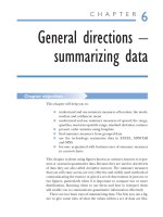
Plot these and use the graph to estimate the internal rate of return for the project.
Look carefully at Figure 8.1 and you will see that the plotted line crosses the horizontal
axis about midway between 10 and 15. This suggests that the internal rate of return for
the project, the discount rate that produces a zero net present value, is about 12.5%.
Discount rate (%)
Net present value (£)
510
10,000
Ϫ10,000
8000
Ϫ8000
6000
Ϫ6000
4000
Ϫ4000
2000
Ϫ2000
0
15 20
Figure 8.1
Net present values and discount rates in Example 8.14
At this point you may find it useful to try Review Questions 8.13 to

8.20 at the end of the chapter.
If you want to find out more about investment appraisal, you will
probably find Drury (2000) helpful.
8.3 Using the technology: investment
appraisal in EXCEL
You can use EXCEL to determine the net present values and internal
rates of return of investment projects.
To obtain the net present value of a project enter the discount rate you
wish to use followed by the initial outlay, as a negative amount, then the
annual cash flows from the venture into a single column of the spread-
sheet. We would enter the data from Example 8.11 in the following way:
Note that cell A7 contains the total cash flow in at the end of the fifth
year, the sum of the £20,000 net profit from operating the coach and
the £40,000 the company expects to sell the coach for at the end of the
fifth year.
Once you have entered the data click on the empty cell A8 then click
in the formula bar and type in:
ϭ NPV(A1, A3:A7) ϩ A2
Press Enter or click the green Ί button to the left of the formula bar to
the right of f
x
in the upper part of the screen and the net present value
figure, £8936.18, should appear in cell A8. The answer we reached in
Example 8.11 was £8936. The small difference is the result of rounding.
For an internal rate of return the procedure is very similar, except
that we do not enter a discount rate as we do for a net present value.
The data for the Budisha Bus Company might be entered as overleaf.
Click in cell A7 then click in the formula bar. Type ϭ IRR(A1:A6) in
the formula bar then click the green tick to the left of the formula bar
Chapter 8 Counting the cost – summarizing money variables over time 273

ABC
1 0.1
2 Ϫ120000
3 30000
4 30000
5 30000
6 25000
7 60000
274 Quantitative methods for business Chapter 8
ABC
1 Ϫ120000
2 30000
3 30000
4 30000
5 25000
6 60000
and 13%, the internal rate of return to the nearest per cent, should
appear in cell A7.
8.4 Road test: Do they really use
investment appraisal?
The origins of the discounting methods of investment appraisal, net
present value and internal rate of return go back some time. Parker
(1968) identifies the concept of present value in the appendix to a set
of interest tables published by the Dutch mathematician Simon Stevin
in 1582. Tables like those produced by Stevin were used extensively by
the banking and insurance companies of the time.
Discounting in the assessment of industrial as against financial invest-
ment begin considerably later, and specifically in the UK railway industry.
Many pioneers, such as Brunel, assumed that once built, railways would
last so long that there was no need to worry about investing in the

replacement and upgrading of track. Within twenty or so years of the
first passenger railway journeys it was clear to Captain Mark Huish,
General Manager of the London and North Western Railway, that as
locomotives and wagons became heavier, trains longer and journeys
more frequent the original track was wearing out faster than anticipated.
In 1853 Huish and two colleagues produced a report on the invest-
ment needs the company ought to address. In making their calcula-
tions they determined
the annual reserve which, at either 4 or 4
1
⁄2 per cent compound
interest, would be necessary in order to reproduce, at the end of the
period, the total amount required to restore the [rail]road. (Huish
et al., 1853, p. 273)
Chapter 8 Counting the cost – summarizing money variables over time 275
Rail companies had to make large-scale investments that paid off
over long periods. Weighing up the returns against the original invest-
ment was no simple matter. Similar concerns arose in the South African
gold mining industry in the early twentieth century. Frankel reported
that:
The present value criterion was applied in the first attempt to measure
the return to capital invested in the Witwatersrand gold mining
industry […] on behalf of the Mining Industry Commission of 1907/8.
(Frankel, 1967, p. 10)
Later in the twentieth century engineers working in capital-intensive
industries, primarily oil and chemicals, developed and applied discount-
ing approaches to investment decisions. Johnson and Kaplan (1991)
refer to three major US oil companies (ARCO, Mobil and Standard
Oil of Indiana) where this occurred, and Weaver and Reilly (1956) of
the Atlas Powder Company of Delaware were advocates in the chemical

industry.
Recent surveys of company practice suggest that both net present
value and internal rate of return are widely used. In his 1992 survey of
UK companies Pike (1996) discovered that 81% used internal rate of
return and 74% used net present value. The equivalent figures in his
survey of usage in 1980 were 57% and 39% respectively.
In a study of large US industrial companies Klammer et al. (1991)
found that the great majority (80% or so) used discounting in apprais-
ing investment in the expansion of existing operations and in the set-
ting up of new operations and operations abroad.
Review questions
Answers to these questions, including fully worked solutions to the Key
questions marked with an asterisk (*), are on pages 649–651.
8.1 An oil refining company buys crude oil to process in its refiner-
ies. The price they have paid per barrel has been:
Year 1997 1999 2001 2003
Cost ($) 22 13 28 25
(a) Calculate a simple price index for
(i) the price in 2003 relative to 1997
(ii) the price in 2001 relative to 1997
(iii) the price in 2003 relative to 1999
(iv) the price in 2001 relative to 1999
(b) Compare your answers to (a) (i) and (ii) with your answers
to (a) (iii) and (iv).
8.2* An office manager purchases regular supplies of paper and toner
for the photocopier. The prices of these supplies (in £) over the
years 2001 to 2003 were:
2001 2002 2003
Paper (per 500 sheets) 9.99 11.99 12.99
Toner (per pack) 44.99 48.99 49.99

Calculate a simple aggregate price index for the prices in 2002
and 2003 using 2001 as the base period.
8.3 A pizza manufacturer purchases cheese, pepperoni and tomato
paste. The prices of these ingredients in 1999, 2001 and 2003
were:
1999 2001 2003
Cheese (per kg) £1.75 £2.65 £3.10
Pepperoni (per kg) £2.25 £2.87 £3.55
Tomato paste (per litre) £0.60 £1.10 £1.35
(a) Calculate a simple aggregate price index for the prices in
2001 and 2003 using 1999 as the base period.
(b) What additional information would you need in order to
calculate a weighted aggregate price index to measure these
price changes?
8.4* Zackon Associates, international corporate lawyers, use both
email and fax to transmit documents. The company account-
ant has worked out that the price of sending a document by fax
has increased from £0.25 in 1998 to £0.45 in 2003. The price of
sending a document by email has increased from £0.50 in 1998
to £0.60 in 2003.
In 1998 the company sent 23,000 documents by fax and 1500
documents by email. In 2003 they sent 12,000 documents by
fax and 15,000 by email.
(a) Calculate the weighted aggregate price index for the prices
in 2003 based on the prices in 1998 using the Laspeyre
method.
(b) Calculate the weighted aggregate price index for 2003
with 1998 as the base year using the Paasche method.
276 Quantitative methods for business Chapter 8
(c) Compare the answers you get for (a) and (b). Which method

would be more appropriate in this case, and why?
8.5 A cab driver pays for fuel, vehicle servicing and maintenance
every 3 months, and an annual operating licence. The prices of
these in 2003 and in 1999, together with the quantity of each
that was purchased during 1999, are:
Price in Price in Quantity bought
2003 (£) 1999 (£) in 1999
Fuel (litre) 0.76 0.48 4100
Servicing (visit) 115.00 83.00 4
Licence 750.00 500.00 1
(a) Calculate the weighted aggregate price index for the prices
in 2003 based on the prices in 1999 using the Laspeyre
method.
(b) In 2003 the driver purchased 4000 litres of fuel, had
the vehicle serviced 4 times and bought the annual licence.
Use these figures to calculate the weighted aggregate price
index for 2003 with 1999 as the base year using the Paasche
method.
(c) Compare the results to (a) and (b) and advise the driver,
who is not good at keeping records, which method of assess-
ing overall changes in costs would be more suitable.
8.6 A textile manufacturer makes casual jackets. The company
buys lining fabric, interfacing fabric and outer fabric. These
fabrics are cut and machined to make the garments. The
prices per metre of these materials in 2001, 2002 and 2003
were:
2001 2002 2003
Lining £2.20 £2.30 £2.35
Interfacing £0.92 £0.95 £1.00
Outer £6.50 £7.25 £7.95

In 2001 the company purchased 2500 metres of lining fabric,
400 metres of interfacing fabric and 2750 metres of outer fab-
ric.In 2002 these quantities were 2800, 500 and 3200 respec-
tively. In 2003 they were 3000, 500 and 5000 respectively.
(a) Calculate Laspeyre price indices for 2002 and 2003 using
2001 as the base period.
Chapter 8 Counting the cost – summarizing money variables over time 277
(b) Calculate Paasche price indices for 2002 and 2003 using
2001 as the base period.
(c) Compare your answers to (a) and (b) and account for any
differences between the values of the price indices.
8.7 A confectioner buys cocoa, cocoa butter, sugar and milk solids.
The prices per kilogram of these ingredients in 1997, 2000 and
2003 were:
1997 2000 2003
Cocoa £1.50 £1.45 £1.70
Cocoa butter £1.30 £1.95 £2.05
Sugar £0.45 £0.50 £0.55
Milk solids £0.35 £0.62 £0.68
The quantities that were purchased in 1997 were 7500 kg of
cocoa, 4200 kg, of cocoa butter, 12,000 kg of sugar and 5700 kg of
milk solids. The purchased amounts of these items in 2000 were
8000 kg, 4000 kg, 13,000 kg and 6000 kg respectively. In 2003
they were 8800 kg, 3100 kg, 15,000 kg and 4500 kg respectively.
(a) Compile Laspeyre price indices for 2000 and 2003 using
1997 as the base year.
(b) Compile Paasche price indices for 2000 and 2003 using
1997 as the base year.
(c) Compare your results for (a) and (b) suggesting reasons
for any differences between them.

8.8* The turnover figures provided in the annual accounts of a
large retail grocer over the six years from 1998 to 2003 were:
Year 1998 1999 2000 2001 2002 2003
Turnover (£m) 7022 7101 7350 7844 8249 8598
The values of the Retail Price Index (RPI) for this period were:
Year 1998 1999 2000 2001 2002 2003
RPI 162.9 165.4 170.3 173.3 176.2 181.3
Use the RPI values to deflate the turnover figures so that they
are all expressed in 1998 pounds.
8.9 An enthusiast paid £5000 for a classic car in 1993. Since that
time the car has been kept carefully and been valued every two
years. The valuations were:
Year 1995 1997 1999 2001 2003
Valuation (£) £5800 £5200 £5500 £6200 £6000
278 Quantitative methods for business Chapter 8
The values of the Retail Price Index (RPI) for these years were:
Year 1995 1997 1999 2001 2003
RPI 149.1 157.5 165.4 173.3 181.3
Use the values of the RPI to adjust the valuations of the car so that
they are all expressed in 1993 pounds. The value of the RPI in
1993 was 140.7.
8.10 A media and entertainments company operates two theme
parks in two different countries: Dorrogoy and Stoymost. The
annual profits of each theme park over the first five years of
operations, in millions of units of local currency (the Lukar in
Dorrogoy and the Diyengi in Stoymost) were:
1998 2003
Dorrogoy (m Lukars) 46.1 182.2
Stoymost (m Diyengi) 15.2 51.4
The governments of the two countries each monitor the general

level of prices using a weighted aggregate price index. Values of
these indices for the years 1998 and 2003 are:
1998 2003
Dorrogoy 112.7 281.4
Stoymost 103.4 192.3
(a) Deflate the profits for Dorrogoy so that the profit figures
are expressed in 1998 Lukars.
(b) Deflate the profits for Stoymost so that the profit figures
are expressed in 1998 Diyengi.
(c) Compare the results you obtain for (a) and (b), and com-
ment on the relative success of the two theme parks over
the period 1998 to 2003.
8.11 Select the appropriate definition for each term on the left-
hand side from the list on the right-hand side.
(i) a simple price index (a) uses current period weights
(ii) a Laspeyre price index (b) an un-weighted index of
prices of several items
(iii) the base period (c) using an index to adjust for
inflation
(iv) the Retail Price Index (d) measures the changes in
the price of one item
Chapter 8 Counting the cost – summarizing money variables over time 279