Quantitative Methods for Business chapter 10 pot

CHAPTER
Is it worth the risk? –
introducing probability
10
Chapter objectives
This chapter will help you to:
■ measure risk and chance using probability
■ recognize the types of probability
■ use Venn diagrams to represent alternatives and combinations
■ apply the addition rule of probability: chances of alternatives
■ apply the multiplication rule of probability: chances of
combinations
■ calculate and interpret conditional probabilities and apply
Bayes’ rule
■ construct and make use of probability trees
■ become acquainted with business uses of probability
This chapter is intended to introduce you to the subject of probability,
the branch of mathematics that is about finding out how likely real
events or theoretical results are to happen. The subject originated in
gambling, in particular the efforts of two seventeenth-century French
mathematical pioneers, Fermat and Pascal, to calculate the odds of cer-
tain results in dice games.
Probability may well have remained a historical curiosity within math-
ematics, little known outside casinos and race-tracks, if it were not for
the fact that probability has proved to be invaluable in fields as varied
as psychology, economics, physical science, market research and medi-
cine. In these and other fields, probability offers us a way of analysing
Chapter 10 Is it worth the risk? – introducing probability 317
chance and allowing for risk so that it can be taken into account
whether we are investigating a problem or trying to make a decision.
Probability makes the difference between facing uncertainty and cop-

ing with risk. Uncertainty is a situation where we know that it is possible
that things could turn out in different ways but we simply don’t know
how probable each result is. Risk, on the other hand, is when we know
there are different outcomes but we also have some idea of how likely
each one is to occur.
Business organizations operate in conditions that are far from cer-
tain. Economic circumstances change, customer tastes shift, employees
move to other jobs. New product development and investment projects
are usually rather a gamble.
As well as these examples of what we might call normal commercial
risk, there is the added peril of unforeseen risk. Potential customers in
developing markets may be ravaged by disease, an earthquake may
destroy a factory, strike action may disrupt transport etc.
The topics you will meet in this chapter will help you to understand
how organizations can measure and assess the risks they have to deal
with. But there is a second reason why probability is a very important
part of your studies: because of the role it plays in future statistical
work.
Almost every statistical investigation that you are likely to come
across during your studies and in your future career, whether it is to
research consumer behaviour, employee attitudes, product quality, or
any other facet of business, will have one important thing in common;
it will involve the collection and analysis of a sample of data.
In almost every case both the people who commission the research
and those who carry it out want to know about an entire population.
They may want to know the opinions of all customers, the attitudes of
all employees, the characteristics of all products, but it would be far too
expensive or time-consuming or simply impractical to study every item
in a population. The only alternative is to study a sample and use the
results to gain some insight into the population.

This can work very well, but only if we have a sample that is random
and we take account of the risks associated with sampling.
A sample is called a random sample if every item in the population
has the same chance of being included in the sample as every other
item in the population. If a sample is not random it is of very little use
in helping us to understand a population.
Taking samples involves risk because we can take different random
samples from a single population. These samples will be composed of
different items from the population and produce different results.
318 Quantitative methods for business Chapter 10
Some samples will produce results very similar to those that we would
get from the population itself if we had the opportunity to study all of
it. Other samples will produce results that are not typical of the popu-
lation as a whole.
To use sample results effectively we need to know how likely they are
to be close to the population results even though we don’t actually
know what the population results are. Assessing this involves the use of
probability.
10.1 Measuring probability
A probability, represented by capital P, is a measure of the likelihood of
a particular result or outcome. It is a number on a scale that runs from
zero to one inclusive, and can be expressed as a percentage.
If there is a probability of zero that an outcome will occur it means
there is literally no chance that it will happen. At the other end of the
scale, if there is a probability of one that something will happen, it
means that it is absolutely certain to occur. At the half-way mark, a
probability of one half means that a result is equally likely to occur as
not to occur. This probability literally means there is a fifty-fifty chance
of getting the result.
So how do we establish the probability that something happens? The

answer is that there are three distinct approaches that can be used to
attach a probability to a particular outcome. We can describe these as
the judgemental, experimental and theoretical approaches to identifying
probabilities.
The judgemental approach means evaluating the chance of some-
thing happening on the basis of opinion alone. Usually the something
is relatively uncommon, which rules out the use of the experimental
approach, and doesn’t occur within a context of definable possibilities,
which rules out the use of the theoretical approach. The source of the
opinion on which the probability is based is usually an expert.
You will often find judgemental probabilities in assessments of polit-
ical stability and economic conditions, perhaps concerning investment
prospects or currency fluctuations. You could, of course, use a judge-
mental approach to assessing the probability of any outcome even
when there are more sophisticated means available. For instance, some
people assess the chance that a horse wins a race solely on their opinion
of the name of the horse instead of studying the horse’s record or ‘form’.
If you use the horse’s form to work out the chance that it wins a race
you would be using an experimental approach, looking into the results
Chapter 10 Is it worth the risk? – introducing probability 319
of the previous occasions when the ‘experiment’, in this case the horse
entering a race, was conducted. You could work out the number of
races the horse has won as a proportion of the total number of races it
has entered. This is the relative frequency of wins and can be used to esti-
mate the probability that the horse wins its next race.
A relative frequency based on a limited number of experiments is
only an estimate of the probability because it approximates the ‘true’
probability, which is the relative frequency based on an infinite num-
ber of experiments.
Of course Example 10.1 is a simplified version of what horse racing

pundits actually do. They would probably consider ground conditions,
other horses in the race and so on, but essentially they base their assess-
ment of a horse’s chances on the experimental approach to setting
probabilities.
There are other situations when we want to establish the probability
of a certain result of some process and we could use the experimental
approach. If we wanted to advise a car manufacturer whether they
should offer a three-year warranty on their cars we might visit their
dealers and find out the relative frequency of the cars that needed
major repairs before they were three years old. This relative frequency
would be an estimate of the probability of a car needing major repair
before it is three years old, which the manufacturer would have to pay
for under a three-year warranty.
We don’t need to go to the trouble of using the experimental
approach if we can deduce the probability using the theoretical
Example 10.1
The horse ‘Starikaziole’ has won 6 of the 16 races it entered. What is the probability that
it will win its next race?
The relative frequency of wins is the number of wins, six, divided by the total number
of races, sixteen:
We can conclude therefore that on the basis of its record, the probability that this
horse wins its next race:
P(Starikaziole wins its next race) ϭ 0.375
In other words, better than a one-third or a one in three chance.
Relative frequency
6
1
6
0.375 or 37.5%ϭϭ
320 Quantitative methods for business Chapter 10

approach. You can deduce the probability of a particular outcome if
the process that produces it has a constant, limited and identifiable
number of possible outcomes, one of which must occur whenever the
process is repeated.
There are many examples of this sort of process in gambling, includ-
ing those where the number of possible outcomes is very large indeed,
such as in bingo and lotteries. Even then, the number of outcomes is
finite, the possible outcomes remain the same whenever the process
takes places, and they could all be identified if we had the time and
patience to do so.
Probabilities of specific results in bingo and lotteries can be deduced
because the same number of balls and type of machine are used each
time. In contrast, probabilities of horses winning races can’t be deduced
because horses enter only some races, the length of races varies and so on.
Example 10.2
A ‘Wheel of Fortune’ machine in an amusement arcade has forty segments. Five of the
segments would give the player a cash prize. What is the probability that you win a cash
prize if you play the game?
To answer this we could build a wheel of the same type, spin it thousands of times and
work out what proportion of the results would have given us a cash prize. Alternatively, we
could question people who have played the game previously and find out what proportion
of them won a cash prize. These are two ways of finding the probability experimentally.
It is far simpler to deduce the probability. Five outcomes out of a possible forty would
give us a cash prize so:
This assumes that the wheel is fair, in other words, that each outcome is as likely to
occur as any other outcome.
P(cash prize)
5
40
0.125 or 12.5%ϭϭ

Gambling is a rich source of illustrations of the use of probabilities
because it is about games of chance. However, it is by no means the
only field where you will find probabilities. Whenever you buy insur-
ance you are buying a product whose price has been decided on the
basis of the rigorous and extensive use of the experimental approach
to finding probabilities.
At this point you may find it useful to try Review Questions 10.1 to
10.3 at the end of the chapter.
Chapter 10 Is it worth the risk? – introducing probability 321
10.2 The types of probability
So far the probabilities that you have met in this chapter have been
what are known as simple probabilities. Simple probabilities are prob-
abilities of single outcomes. In Example 10.1 we wanted to know the
chance of the horse winning its next race. The probability that the horse
wins its next two races is a compound probability.
A compound probability is the probability of a compound or com-
bined outcome. In Example 10.2 winning a cash prize is a simple out-
come, but winning cash or a non-cash prize, like a cuddly toy, is a
compound outcome.
To illustrate the different types of compound probability we can
apply the experimental approach to bivariate data. We can estimate
compound probabilities by finding appropriate relative frequencies
from data that have been tabulated by categories of attributes, or
classes of values of variables.
Example 10.3
The Shirokoy Balota shopping mall has a food hall with three fast food outlets;
Bolshoyburger, Gatovielle and Kuriatina. A survey of transactions in these establish-
ments produced the following results.
What is the probability that the customer profile is Family?
What is the probability that a transaction is in Kuriatina?

These are both simple probabilities because they each relate to only one variable –
customer profile in the first case, establishment used in the second.
According to the totals column on the right of the table, in 131 of the 500 transac-
tions the customer profile was Family, so
which is the relative frequency of Family customer profiles.
P(Family)
131
500
0.262 or 26.2%ϭϭ
Customer profile Bolshoyburger Gatovielle Kuriatina Total
Lone 87 189 15 291
Couple 11 5 62 78
Family 4 12 115 131
Total 102 206 192 500
322 Quantitative methods for business Chapter 10
If we want to use a table such as in Example 10.3 to find compound
probabilities we must use figures from the cells within the table, rather
than the column and row totals, to produce relative frequencies.
It is laborious to write full descriptions of the outcomes so we can
abbreviate them. We will use ‘L’ to represent Lone customers, ‘C ’ to rep-
resent Couple customers and ‘F ’ for Family customers. Similarly, we will
use ‘B’ for Bolshoyburger, ‘G ’ for Gatovielle and ‘K’ for Kuriatina. So we
can express the probability in Example 10.4 in a more convenient way.
P(Lone customer profile and Bolshoyburger purchase) ϭ P(L and B)
ϭ 0.174
The type of compound probability in Example 10.4, which includes
the word ‘and’, measures the chance of the intersection of two out-
comes. The relative frequency we have used as the probability is based
on the number of people who are in two specific categories of the ‘cus-
tomer profile’ and ‘establishment’ characteristics. It is the number of

people who are at the ‘cross-roads’ or intersection between the ‘Lone’
and the ‘Bolshoyburger’ categories.
Finding the probability of an intersection of two outcomes is quite
straightforward if we apply the experimental approach to bivariate
data. In other situations, for instance where we only have simple prob-
abilities to go on, we need to use the multiplication rule of probability,
which we will discuss later in the chapter.
Example 10.4
What is the probability that the profile of a customer in Example 10.3 is Lone and
their purchase is from Bolshoyburger?
The number of Lone customers in the survey who made a purchase from
Bolshoyburger was 87 so:
P(Lone customer profile and Bolshoyburger purchase)
Similarly, from the totals row along the bottom of the table, we find that 192 of the
transactions were in Kuriatina, so
which is the relative frequency of transactions in Kuriatina.
P(Kuriatina)
192
500
0.384 or 38.4%ϭϭ
87
500
0.174 or 17.4%ϭϭ
There is a second type of compound probability, which measures the
probability that one out of two or more alternative outcomes occurs.
This type of compound probability includes the word ‘or’ in the
description of the outcomes involved.
The type of compound probability in Example 10.5 measures the
chance of a union of two outcomes. The relative frequency we have
used as the probability is based on the combined number of transac-

tions in two specific categories of the ‘customer profile’ and ‘establish-
ment’ characteristics. It is the number of transactions in the union or
‘merger’ between the ‘Couple’ and the ‘Kuriatina’ categories.
To get a probability of a union of outcomes from other probabilities,
rather than by applying the experimental approach to bivariate data,
we use the addition rule of probability. You will find this discussed later
in the chapter.
Chapter 10 Is it worth the risk? – introducing probability 323
Example 10.5
Use the data in Example 10.3 to find the probability that a transaction involves a Couple
or is in Kuriatina.
The probability that one (and by implication, both) of these outcomes occurs is
based on the relative frequency of the transactions in one or other category. This
implies that we should add the total number of transactions at Kuriatina to the total
number of transactions involving customers profiled as Couple, and divide the result by
the total number of transactions in the survey.
Number of transactions at Kuriatina ϭ 15 ϩ 62 ϩ 115 ϭ 192
Number of transactions involving Couples ϭ 11 ϩ 5 ϩ 62 ϭ 78
Look carefully and you will see that the number 62 appears in both of these expres-
sions. This means that if we add the number of transactions at Kuriatina to the number
of transactions involving Couples to get our relative frequency figure we will double-
count the 62 transactions involving both Kuriatina and Couples. The probability we get
will be too large.
The problem arises because we have added the 62 transactions by Couples at
Kuriatina in twice. To correct this we have to subtract the same number once.
PK C( or )
(15 62 115) (11 5 62) 62 192 78 62
208
500
0.416 or 41.6%

ϭ
ϩϩ ϩϩϩϪ
ϭ
ϩϪ
ϭϭ
500 500
324 Quantitative methods for business Chapter 10
The third type of compound probability is the conditional probability.
Such a probability measures the chance that one outcome occurs given
that, or on condition that, another outcome has already occurred.
At this point you may find it useful to try Review Questions 10.4 to
10.9 at the end of the chapter.
It is always possible to identify compound probabilities directly from
the sort of bivariate data in Example 10.3 by the experimental
approach. But what if we don’t have this sort of data? Perhaps we have
some probabilities that have been obtained judgementally or theoret-
ically and we want to use them to find compound probabilities. Perhaps
there are some probabilities that have been obtained experimentally
but the original data are not at our disposal. In such circumstances we
need to turn to the rules of probability.
10.3 The rules of probability
In situations where we do not have experimental data to use we
need to have some method of finding compound probabilities. There
are two rules of probability: the addition rule and the multiplica-
tion rule.
Example 10.6
Use the data in Example 10.3 to find the probability that a transaction in Gatovielle
involves a Lone customer.
Another way of describing this is that given (or on condition) that the transaction is
in Gatovielle, what is the probability that a Lone customer has made the purchase. We

represent this as:
P(L|G)
Where ‘|’ stands for ‘given that’.
We find this probability by taking the number of transactions involving Lone cus-
tomers as a proportion of the total number of transactions at Gatovielle.
This is a proportion of a subset of the 500 transactions in the survey. The majority of
them, the 294 people who did not use Gatovielle, are excluded because they didn’t
meet the condition on which the probability is based, i.e. purchasing at Gatovielle.
PLG(|)
189
206
0.9175 or 91.75%ϭϭ
Chapter 10 Is it worth the risk? – introducing probability 325
10.3.1 The addition rule
The addition rule of probability specifies the procedure for finding the
probability of a union of outcomes, a compound probability that is
defined using the word ‘or’.
According to the addition rule, the compound probability of one or
both of two outcomes, which we will call A and B for convenience, is
the simple probability that A occurs added to the simple probability
that B occurs. From this total we subtract the compound probability
of the intersection of A and B, the probability that both A and B occur.
That is:
P(A or B) ϭ P(A) ϩ P(B) Ϫ P(A and B)
Example 10.7
Use the addition rule to calculate the probability that a transaction in the food hall in
Example 10.3 is at Kuriatina or involves a Couple.
Applying the addition rule:
P(K or C) ϭ P(K) ϩ P(C) Ϫ P(K and C)
The simple probability that a transaction is at Kuriatina:

The simple probability that a transaction involves a Couple:
The probability that a transaction is at Kuriatina and involves a Couple:
So:
PK C( or )
192
500
78
500
62
500
192 78 62 208
500
0.416 or 41.6%
ϭϩϪ
ϭ
ϩϪ
ϭϭ
500
PK C( and )
62
500
ϭ
PC()
78
500
ϭ
PK()
192
500
ϭ

If you compare this answer to the answer we obtained in Example 10.5
you will see they are exactly the same. In this case the addition rule is
an alternative means of getting to the same result. In some ways it is
more convenient because it is based more on row and column totals of
326 Quantitative methods for business Chapter 10
the table in Example 10.3 rather than numbers from different cells
within the table.
The addition rule can look more complicated than it actually is
because it is called the addition rule yet it includes a subtraction. It may
help to represent the situation in the form of a Venn diagram, the sort
of diagram used in part of mathematics called set theory.
In a Venn diagram the complete set of outcomes that could occur,
known as the sample space, is represented by a rectangle. Within the rect-
angle, circles are used to represent sets of outcomes.
In Figure 10.1 the circle on the left represents the Kuriatina transac-
tions, and the circle on the right represents the Couple transactions.
The area covered by both circles represents the probability that a trans-
action is at Kuriatina or involves a Couple. The area of overlap repre-
sents the probability that a transaction is both at Kuriatina and involves
a Couple. The area of the rectangle outside the circles contains trans-
actions that are not at Kuriatina and do not involve Couples.
By definition the area of overlap is part of both circles. If you simply
add the areas of the two circles together to try to get the area covered
by both circles, you will include the area of overlap twice. If you sub-
tract it once from the sum of the areas of the two circles you will only
have counted it once.
The addition rule would be simpler if there were no overlap; in other
words, there is no chance that the two outcomes can occur together.
This is when we are dealing with outcomes that are known as mutually
exclusive. The probability that two mutually exclusive outcomes both

occur is zero.
In this case we can alter the addition rule:
P(A or B) ϭ P(A) ϩ P(B) Ϫ P(A and B)
KC
Figure 10.1
A Venn diagram
to illustrate
Example 10.7
Chapter 10 Is it worth the risk? – introducing probability 327
to P(A or B) ϭ P(A) ϩ P(B)
because P(A and B) ϭ 0.
Example 10.9
What is the probability that one of the prospective car-buyers in Example 10.8 chooses
the ‘Almiak’ or the ‘Balanda’ or the ‘Caverza’ or chooses not to take a test drive? For
convenience we will use the letter N to denote the latter.
The simple probability that a prospective car-buyer picks the ‘Almiak’ ϭ
PA()
43
178
ϭ
Example 10.8
One weekend a total of 178 prospective car-buyers visit a car showroom. They are
offered the chance to test drive one of three vehicles: the off-road ‘Almiak’, the
‘Balanda’ saloon, or the ‘Caverza’ sports car. When invited to select the car they would
like to drive, 43 chose the ‘Almiak’, 61 the ‘Balanda’ and 29 the ‘Caverza’.
What is the probability that a prospective car-buyer from this group has chosen the
‘Balanda’ or the ‘Caverza’?
We can assume that the choices are mutually exclusive because each prospective buyer
can only test drive one car. We can therefore use the simpler form of the addition rule.
For convenience we can use the letter A for ‘Almiak’, B for ‘Balanda’ and C for

‘Caverza’.
PB C PB PC( or ) ( ) ( )
61
178
29
178
90
178
0.5056 or 50.56%ϭ ϩϭϩϭϭ
If you read Example 10.8 carefully you can see that although the
three choices of car are mutually exclusive, they do not constitute all of
the alternative outcomes. That is to say, they are not collectively exhaus-
tive. As well as choosing one of the three cars each prospective car-
buyer has a fourth choice, to decline the offer of a test drive. If you
subtract the number of prospective car-buyers choosing a car to drive
from the total number of prospective car-buyers you will find that 45 of
the prospective car-buyers have not chosen a car to drive.
A footnote to the addition rule is that if we have a set of mutually exclu-
sive and collectively exhaustive outcomes their probabilities must add up
to one. A probability of one means certainty, which reflects the fact that
in a situation where there are a set of mutually exclusive and collectively
exhaustive outcomes, one and only one of them is certain to occur.
328 Quantitative methods for business Chapter 10
This footnote to the addition rule can be used to derive probabilities of
one of a set of mutually exclusive and collectively exhaustive outcomes
if we know the probabilities of the other outcomes.
The result we obtained in Example 10.10, 0.2528, is the decimal equiva-
lent of the figure of 45/178 that we used for P(N) in Example 10.9.
10.3.2 The multiplication rule
The multiplication rule of probability is the procedure for finding the

probability of an intersection of outcomes, a compound probability
that is defined using the word ‘and’.
According to the multiplication rule the compound probability that
two outcomes both occur is the simple probability that the first one
occurs multiplied by the conditional probability that the second out-
come occurs, given that the first outcome has already happened:
P(A and B) ϭ P(A)*P(B|A)
Example 10.10
Deduce the probability that a prospective car-buyer in Example 10.8 declines to take a
test drive using the simple probabilities of the other outcomes.
PPAPBPC(Prospective car - buyer declines a test drive) 1 ( ) ( ) ( )
1
43
178
61
178
29
178
1 0.2416 0.3427 0.1629
1 0.7472 0.2528 or 25.28%
ϭϪϪϪ
ϭϪϪϪ
ϭϪϪϪ
ϭϪ ϭ
The simple probability that a prospective car-buyer picks the ‘Balanda’ ϭ
The simple probability that a prospective car-buyer picks the ‘Caverza’ ϭ
The simple probability that a prospective car-buyer declines a test drive ϭ
PA B C N( or or or )
43 61 29 45 178
178

1ϭ
ϩϩϩ
ϭϭ
178
PN()
45
1
78
ϭ
PC()
29
1
78
ϭ
PB()
61
17
8
ϭ
Chapter 10 Is it worth the risk? – introducing probability 329
The multiplication rule is what bookmakers use to work out odds for
‘accumulator’ bets, bets that a sequence of outcomes, like several spe-
cific horses winning races, occurs. To win the bet the first horse must
win the first race; the second horse must win the second race and so on.
The odds of this sort of thing happening are often something like five
hundred to one. The numbers, like five hundred, are large because
they are obtained by multiplication.
Example 10.11
Use the multiplication rule to calculate the probability that a transaction at the food
hall in Example 10.3 involved a Lone customer and was at Bolshoyburger.

P(L and B) ϭ P(L) * P(B|L)
From the table in Example 10.3:
which is the relative frequency of transactions involving a Lone customer
and
which is the relative frequency of transactions involving Lone customers that were at
Bolshoyburger.
So
PL B( and )
291
500
*
87
291
0.582 * 0.299 0.174 or 17.4%ϭϭ ϭ
PBL( | )
87
291
ϭ
PL()
291
500
ϭ
If you compare this figure to the answer we obtained in Example 10.4
you will see that they are exactly the same.
The multiplication rule can look more complex than it actually is
because it includes a conditional probability. We use a conditional
probability for the second outcome because the chances of it occur-
ring could be influenced by the first outcome. This is called dependency;
in other words, one outcome is dependent on the other.
You can find out whether two outcomes are dependent by compar-

ing the conditional probability of one outcome given that the other
has happened, with the simple probability that it happens. If the two
figures are different, the outcomes are dependent.
The multiplication rule can be rearranged to provide us with a way
of finding a conditional probability:
if P(A and B) ϭ P(A) * P(B|A)
then if we divide both sides by P(A) we get
so
PBA
PA B
PA
( | )
( and )
ϭ
()
PA B
PA
PBA
( and )
()
(|)ϭ
330 Quantitative methods for business Chapter 10
Example 10.13
What is the probability that a transaction at Gatovielle in the food hall in Example 10.3
involves a Lone customer?
From the table in Example 10.3
and
so
PLG( | )
0.378

0.412
0.9175 or 91.75%ϭϭ
PG()
206
500
0.412ϭϭ
PL G( and )
189
500
0.378ϭϭ
PLG
PL G
PG
( | )
( and )
ϭ
()
Example 10.12
At a promotional stall in a supermarket shoppers are invited to taste ostrich meat.
A total of 200 people try it and 122 of them say they liked it. Of these, 45 say they would
buy the product. Overall 59 of the 200 shoppers say they would buy the product.
Are liking the product and expressing the intention to buy it dependent?
The simple probability that a shopper expresses an intention to buy is 59/200 or 29.5%.
The conditional probability that a shopper expresses an intention to buy given that
they liked the product is 45/122 or 36.9%.
There is a difference between these two figures, which suggests that expressing an
intention to buy is dependent on liking the product.
Chapter 10 Is it worth the risk? – introducing probability 331
You might like to compare this to the answer we obtained in
Example 10.6, which is exactly the same.

If there had been no difference between the two probabilities in
Example 10.12 there would be no dependency; that is, the outcomes
would be independent. In situations where outcomes are independent, the
conditional probabilities of the outcomes are the same as their simple
probabilities. This means we can simplify the multiplication rule when
we are dealing with independent outcomes. We can replace the condi-
tional probability of the second outcome given that the first outcome has
occurred with the simple probability that the second outcome occurs.
That is:
instead of P(A and B) ϭ P(A) * P(B|A)
we can use P(A and B) ϭ P(A) * P(B)
because P(B) ϭ P(B|A).
Example 10.15
Bella is taking her friend out for the evening but has forgotten to take some cash out of
her bank account. She reaches the cash machine, but can’t remember the exact
Example 10.14
What is the probability that a player who plays the Wheel of Fortune in Example 10.2
twice, wins cash prizes both times?
Five of the forty segments give a cash prize, so the probability of a cash prize in any
one game is 5/40.
The conditional probability that a player gets a cash prize in their second game given
that they have won a cash prize in their first game is also 5/40. The outcomes are inde-
pendent; in other words, the result of the second game is not influenced, or conditioned
by the result of the first. (If this is not clear because you feel there is a connection, you
might ask yourself how the Wheel of Fortune remembers what it did the first time!)
We will use the letter C to represent a cash prize. The first cash prize the player wins
can then be represented as C
1
, and the second as C
2

.
PC C PC PC( and ) ( ) * ( )
5
40
*
5
40
0.016 or 1.6%
12
ϭϭϭ
Conditional probabilities are particularly important if you want to
work out the chance of a sequence of outcomes involving a limited
number of elements. In these cases the selection of one of the elem-
ents alters the probabilities of further selections.
332 Quantitative methods for business Chapter 10
At this point you may find it useful to try Review Questions 10.10 to
10.15 at the end of the chapter.
10.3.3 Bayes’ rule
In the last section we looked at how the multiplication rule, which
enables us to find the compound probability that both of two out-
comes occur, could be rearranged to provide a definition of the condi-
tional probability that the second outcome occurs given that the first
outcome had already occurred. That is, if
P(A and B) ϭ P(A) * P(B|A)
then
In this context we normally assume that outcome A occurs before
outcome B, for instance the probability that a person buys a car (B)
given that they have test driven it (A).
Thanks to the work of the eighteenth-century clergyman and math-
ematician Thomas Bayes, we can develop this further to say that:

P(B and A) ϭ P(B) * P(A|B)
so
This means that we can find the probability that outcome A happened
given that we know outcome B has subsequently happened. This is
PAB
PB A
PB
( | )
( and )
()
ϭ
PBA
PA B
PA
( | )
( and )
()
ϭ
sequence of her PIN number. She knows that the digits in her PIN number are 2, 7, 8
and 9. What is the probability that Bella enters the correct PIN number?
There are four digits in Bella’s PIN number so the chance that she keys in the correct
first digit is one chance in four. The conditional probability that, assuming she has keyed
in the correct first digit she then keys in the correct second digit is one in three as there
are three possible digits remaining and only one of them is the correct one. The condi-
tional probability that given she gets the first two right she then keys in the correct third
digit is one in two as she is left with two digits, one of which is the correct one. The con-
ditional probability that she gets the last one right, assuming that she has keyed in the first
correctly is one since there is only one digit left and it must be the correct fourth digit.
P(PIN number correct)
1

4
0.042ϭϭ***
1
3
1
2
1
known as a posterior, or ‘after-the event’ probability. In contrast, the sim-
ple probability that outcome A happens is a prior, or ‘before-the event’
probability.
The compound probability that both A and B occur is the same
whether it is described as the probability of A and B or the probability
of B and A. That is:
P(A and B) ϭ P(B and A)
The multiplication rule tells us that:
P(A and B) ϭ P(A) * P(B|A)
We can therefore express the conditional probability that A has
occurred given that we know B has subsequently occurred as:
This definition of the posterior probability of an outcome is known
as Bayes’ rule or Bayes’ theorem.
PAB
PA PBA
PB
(|)
()*(|)
()
ϭ
Chapter 10 Is it worth the risk? – introducing probability 333
Example 10.16
A financial services ombudsman is investigating the mis-selling of pension schemes

some years previously. Some buyers of these pension schemes were sold the schemes on
the basis of misleading information, and would have been better off had they made
alternative arrangements.
The pension schemes being investigated were provided by one company but actually
sold by two brokers, Copilka, who sold 80% of the schemes, and Denarius, who sold
20% of the schemes. Some of the pension schemes sold by these brokers were appro-
priate for the customers who bought them, but the ombudsman has established that
30% of the schemes sold by Copilka and 40% of the schemes sold by Denarius have
turned out to be inappropriate for the customers who bought them.
The ombudsman wishes to apportion liability for compensation for mis-sold pension
schemes between the two brokers and wants to do so on the basis of the following:
(a) If a pension scheme was mis-sold what is the probability that it was sold by
Copilka?
(b) If a pension scheme was mis-sold what is the probability that it was sold by
Denarius?
We will use M to represent a pension scheme that was mis-sold, C to denote that a
pension scheme was sold by Copilka, and D to denote that a pension scheme was sold
by Denarius.
334 Quantitative methods for business Chapter 10
The first probability that the ombudsman needs to know is P(C |M ).
Using Bayes’ rule:
We know that the probability that a pension scheme was sold by Copilka, P(C), is 0.8.
We also know that the probability that a pension scheme was mis-sold given that it
was sold by Copilka, P(M|C) is 0.3. The only other probability that we need in order
to apply Bayes’ rule in this case is P(M), the probability that a pension scheme was
mis-sold.
A pension scheme that was mis-sold must have been sold by either Copilka or
Denarius. The probability that a pension scheme was mis-sold must therefore be the sum
of the probability that a pension scheme was mis-sold and it was sold by Copilka and the
probability that a pension scheme was mis-sold and it was sold by Denarius. That is:

P(M) ϭ P(C and M) ϩ P(D and M)
Although we do not know these compound probabilities we can derive them by
applying the multiplication rule:
P(C and M ) ϭ P(C) * P(M|C) ϭ 0.8 * 0.3 ϭ 0.24
The probability that a pension scheme was sold by Denarius, P(D) is 0.2, and
the probability that a pension scheme was mis-sold given that it was sold by Denarius,
P(M|D) is 0.4, so:
P(D and M) ϭ P(D) * P(M|D) ϭ 0.2 * 0.4 ϭ 0.08
so P(M) ϭ 0.24 ϩ 0.08 ϭ 0.32
We can now work out the first of the two probabilities that the ombudsman needs;
the probability that if a pension scheme was mis-sold it was sold by Copilka, P(C|M):
A mis-sold pension scheme must have been sold by Denarius if it was not sold by
Copilka, they are mutually exclusive and collectively exhaustive outcomes. This means
that we can deduce that the probability that if a pension scheme was mis-sold it was sold
by Denarius, P(D|M) is one less P(C|M):
P(D|M) ϭ 1 Ϫ 0.75 ϭ 0.25
On the basis of these results the ombudsman should apportion 75% of the liability
for compensation to Copilka and 25% of the liability for compensation to Denarius.
PCM
PC PMC
PM
( | )
( )* ( | ) 0.8 * 0.3
0.24
0.32
0.75ϭϭϭϭ
() .032
PCM
PC PMC
PM

( | )
() * ( |)
ϭ
()
Chapter 10 Is it worth the risk? – introducing probability 335
At this point you may find it useful to try Review Questions 10.16 and
10.17 at the end of the chapter.
10.3.4 Applying the rules of probability
Although we have dealt separately with different types of probability,
rules of probability and so on, when it comes to applying them to solve
problems involving sequences of outcomes you may well have to use
them together. You may like to look at Example 10.17, which brings
together many of the topics that you have met in this chapter to solve
an apparently straightforward problem.
Example 10.17
Twenty-five graduates join a company at the same time. During their training pro-
gramme friendships are established and they decide that when one of them has a birth-
day they will all dine at a restaurant chosen by the person whose birthday is being
celebrated. One of the graduates asks what will happen if two or more of them share a
birthday. In response another says that it won’t happen because there are only 25 of
them and 365 days in the year.
What is the probability that there will be at least one clash of birthdays in a year?
This is quite a complex question because of the sheer variety of ways in which there
could conceivably be a clash of birthdays. We could have a clash on the 1st of January,
the 2nd of January and so on. Maybe three graduates could share the same birthday? It
would be extremely difficult and tedious to work out all these probabilities separately.
In fact we don’t need to. One of the phrases you may remember from the discussion
of the addition rule was ‘mutually exclusive and collectively exhaustive’. Such outcomes
rule each other out and have probabilities that add up to one. We can use this here.
We have two basic outcomes: either some birthdays clash or none do. They are mutu-

ally exclusive because it is impossible to have both clashes and no clashes. They are col-
lectively exhaustive because we must have either clashes or no clashes.
This makes things easier. We want the probability of clashes, but to get that we would
have to analyse many different combinations of outcomes and put their probabilities
together. Instead we can work out the probability than there are no clashes and take it
away from one. This is easier because there is only one probability to work out.
What is the probability that there are no clashes?
Imagine if there was just one graduate and we introduced the others one at a time.
The first graduate can have a birthday on any day; there are no other graduates whose
birthdays could clash.
336 Quantitative methods for business Chapter 10
10.4 Tree diagrams
If you have to investigate the probabilities of sequences of several
outcomes it can be difficult to work out the different combinations of
The probability that the second graduate has a birthday on a different day is 364/365
because one day is already ‘occupied’ by the birthday of the first graduate, leaving 364
‘free’ days.
The probability that the third graduate has a birthday on a different day to the other
two graduates assuming that the first two graduates’ birthdays don’t clash is 363/365.
This is the conditional probability that the third graduate’s birthday misses those of
both the first and second graduates, given that the birthdays of the first and second
graduates don’t clash. The number 363 appears because that is the number of ‘free’
days remaining if the birthdays of the first two graduates don’t clash.
Continuing the process, the probability that the fourth graduate’s birthday doesn’t
clash with those of the first three, assuming the first three are on different days, is
362/365. The probability that the fifth graduate’s birthday doesn’t clash with those of
the first four is 361/365, and so on.
Eventually we reach the probability that the twenty-fifth graduate’s birthday doesn’t
clash with those of the other twenty-four, assuming none of the previous twenty-four
birthdays clash, which is 341/365.

The probabilities that we now have are probabilities that the birthdays of specific
graduates don’t clash with those of other specific graduates. What we want is the prob-
ability that there are no clashes at all. To get this we have to put these probabilities
together. But how? Should we multiply or add?
The answer is that we multiply them together. We want the probability that the sec-
ond graduate’s birthday misses that of the first graduate and the third graduate’s birth-
day misses those of the first two and so on.
So
ϭ 0.4252 or 42.52%
This is the probability that there are no clashes, but we wanted to find the probabil-
ity that there is at least one clash. For this we use the addition rule. It is certain that
there is either at least one clash or no clash:
P(at least one clash) ϩ P(no clash) ϭ 1
So P(at least one clash) ϭ 1 Ϫ P(no clash)
ϭ 1 Ϫ 0.4252 ϭ 0.5748 or 57.48%
P(no clashes)
364
365
ϭ *****
363
365
362
365
342
365
341
365
K
outcomes in your head. It helps if you write down all the different varia-
tions, and you may find a Venn diagram a useful way of arranging them

in order to work out probabilities of certain types of combinations. But
perhaps the best way of sorting out this kind of problem is to use a tree
diagram.
A tree diagram, which is sometimes called a probability tree, repre-
sents the different sequences of outcomes in the style of a tree that
‘grows’ from left to right. Each branch of the tree leads to a particular
result.
On the right hand side of the diagram, at the end of each branch, we
can insert the combination of outcomes that the sequence of branches
represents and, using the multiplication rule, the probability that the
sequence of outcomes happens.
Chapter 10 Is it worth the risk? – introducing probability 337
Example 10.18
Three friends start Higher Education courses at the same time in the same institution.
Armand is studying Architecture, Brendan is studying Banking and Chloe is studying
Chemistry. Seventy per cent of students who begin the Architecture course complete it
successfully, 80% of students who begin the Banking course complete it successfully and
60% of students who begin the Chemistry course complete it successfully. Construct a
tree diagram and use it to work out:
■ The probability that all three friends successfully complete their courses.
■ The probability that two of the friends successfully complete their courses.
■ The probability that only one of the friends successfully completes their
course.
We will use A to represent Armand, B for Brendan and C for Chloe. To indicate some-
one failing their course we will use the appropriate letter followed by a ‘mark, so A’ rep-
resents the outcome that Armand fails his course, whereas A alone represents the
outcome that Armand completes his course successfully.
The completion rate suggests the probability that Armand passes the Architecture
course is 0.7, and given that the ‘pass’ and ‘fail’ outcomes are mutually exclusive and col-
lectively exhaustive, the probability he fails is 0.3. The probability that Brendan passes

the Banking course is 0.8, and the probability that he fails is 0.2. The probability that
Chloe passes the Chemistry course is 0.6 and the probability that she fails is 0.4.
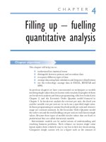
In Figure 10.2 the probability that all three pass, P(ABC), is the probability at the top
on the right-hand side, 0.336 or 33.6%.
The probability that two of the friends pass is the probability that one of three
sequences, either ABCЈ or ABЈC or AЈBC occurs. Since these combinations are mutually
338 Quantitative methods for business Chapter 10
A tree diagram should include all possible sequences. One way you
can check that it does is to add up the probabilities on the right-hand
side. Because these outcomes are mutually exclusive and collectively
exhaustive their probabilities should add up to one. We can check that
this is the case in Example 10.18.
0.336 ϩ 0.224 ϩ 0.084 ϩ 0.056 ϩ 0.144 ϩ 0.096 ϩ 0.036 ϩ 0.024 ϭ 1
At this point you may find it useful to try Review Questions 10.18
and 10.19 at the end of the chapter.
exclusive we can apply the simpler form of the addition rule:
P(ABCЈ or ABЈC or AЈBC) ϭ 0.224 ϩ 0.084 ϩ 0.144 ϭ 0.452 or 45.2 per cent
The probability that only one of the friends passes is the probability that either ABЈCЈ
or AЈBCЈ or AЈBЈC occurs. These combinations are also mutually exclusive, so again we
can apply the simpler form of the addition rule:
P(ABЈCЈ or AЈBCЈ or AЈBЈC) ϭ 0.056 ϩ 0.096 ϩ 0.036 ϭ 0.188 or 18.8 per cent
Outcomes Probability
C ABC 0.7
*
0.8
*
0.6 ϭ 0.336
B
CЈ ABCЈ 0.7
*

0.8
*
0.4 ϭ 0.224
ABЈ CABЈC 0.7
*
0.2
*
0.6 ϭ 0.084
CЈ ABЈCЈ 0.7
*
0.2
*
0.4 ϭ 0.056
CAЈBC 0.3
*
0.8
*
0.6 ϭ 0.144
AЈ BCЈ AЈBCЈ 0.3
*
0.8
*
0.4 ϭ 0.096
BЈ CAЈBЈC 0.3
*
0.2
*
0.6 ϭ 0.036
CЈ AЈBЈCЈ 0.3
*

0.2
*
0.4 ϭ 0.024
Figure 10.2
Tree diagram for Example 10.18
Chapter 10 Is it worth the risk? – introducing probability 339
10.5 Road test: Do they really use
probability?
There is one field of business where the very definition of the products is
probabilities; the betting industry. Whether you want to gamble on a horse
race, bet on which player will score first in a game of football, have a punt
on a particular tennis player winning a grand slam event, you are buying a
chance, a chance which is measured in terms of probability, ‘the odds’.
Another industry delivering products based on probability is the insur-
ance industry. When you buy insurance you are paying the insurer to
meet the financial consequences of any calamity that may be visited upon
you. When you buy motor insurance, for example, you are paying for the
insurance company to cover the costs you might incur if you have an acci-
dent. Clearly the company would be rash to offer you this cover without
weighing up the chances of your having an accident, which is why when
you apply for insurance you have to provide so much information about
yourself and your vehicle. If you don’t have an accident the company
makes a profit from you, if you do it will lose money. Insurance companies
have extensive records of motor accidents. They reference the informa-
tion you give them, your age and gender, the type of car you use, etc.
against their databases to assess the probability of your having an accident
and base the cost of your insurance on this probability.
The legal context within which businesses operate places obligations
on them to ensure their operations do not endanger the health and
safety of their workers, and their products are not harmful to their cus-

tomers or the wider environment. For this reason companies undertake
risk assessments. These assessments typically involve using probability to
define the risks that their activities may pose. Boghani (1990) describes
how probability has been employed in assessing the risks associated with
transporting hazardous materials on special trains. North (1990)
explains how the process of judgemental evaluation was used to ascertain
probabilities of potential damage to forestry production and fish stocks
in the lakes of Wisconsin from sulphur dioxide emissions. In the same
paper North shows how experimental data were used to assess the health
risks arising from the use of a particular solvent in dry-cleaning.
Review questions
Answers to these questions, including fully worked solutions to the Key
questions (marked *), are on pages 656–657.
340 Quantitative methods for business Chapter 10
10.1 An electrical goods retailer sold DVD systems to 8200 cus-
tomers last year and extended warranties to 3500 of these cus-
tomers. When the retailer sells a DVD system, what is the
probability that:
(a) the customer will buy an extended warranty?
(b) the customer will not buy an extended warranty?
10.2 Since it was set up 73,825 people have visited the website of a
music and fashion magazine and 6301 of them purchased goods
on-line. When someone visits the site what is the probability
that:
(a) they do not purchase goods on-line?
(b) they do purchase goods on-line?
10.3 A direct marketing company produces leaflets offering mem-
bership of a book club. These leaflets are then inserted into the
magazine sections of two Sunday newspapers, the Citizen and
the Despatch, 360,000 leaflets being put in copies of the Citizen and

2,130,000 put in copies of the Despatch. The company receives
19,447 completed leaflets from Citizen readers and 58,193
completed leaflets from Despatch readers. What is the prob-
ability that:
(a) a Citizen reader returns a leaflet?
(b) a Despatch reader returns a leaflet?
10.4* A garage offers a breakdown recovery service for motorists
that is available every day of the year. According to their
records the number of call-outs they received per day last year
were:
Number of call-outs 0 1 2 3 4
Number of days 68 103 145 37 12
What is the probability that:
(a) they receive two call-outs in a day?
(b) they receive two or fewer call-outs in a day?
(c) they receive one or more call-outs in a day?
(d) they receive less than four call-outs in a day?
(e) they receive more than two call-outs in a day?
10.5 Last year 12,966 people opened new accounts at a building
society. Of these 5314 were branch-based accounts, 4056 were
postal accounts and 3596 were Internet accounts. What is the
probability that when a customer opens a new account:
(a) it is a postal account?
(b) it is an Internet account?
(c) it is either branch-based or postal?