Quantitative Methods for Business chapter 12 pptx
Bạn đang xem bản rút gọn của tài liệu. Xem và tải ngay bản đầy đủ của tài liệu tại đây (191.38 KB, 31 trang )
CHAPTER
Accidents and
incidence – discrete
probability distributions
and simulation
12
Chapter objectives
This chapter will help you to:
■ work out the probabilities for a basic discrete probability
distribution
■ calculate the mean and standard deviation of a discrete prob-
ability distribution
■ model business processes with the binomial distribution
■ model business processes with the Poisson distribution
■ simulate simple random business processes with random
numbers
■ use the technology: discrete probability distributions in
EXCEL, MINITAB and SPSS, random number generation in
EXCEL
■ become acquainted with business uses of discrete probability
distributions and simulation
Chapter 12 Accidents and incidence – discrete probability distributions and simulation 375
In this chapter we will bring together two key concepts from earlier
chapters. The first of these is the idea of a frequency distribution, which
shows the frequency or regularity with which the values of a variable
occur, in other words how they are distributed across their range. The
second key concept is that of probability, which we considered in
Chapter 9. Here we will be looking at probability distributions which por-
tray not the frequency with which values of a distribution actually occur
but the probability with which we predict they will occur.
Probability distributions are very important tools for modelling or
representing processes that occur at random, such as customers visit-
ing a website or accidents on a building site. These are examples of dis-
crete random variables as they vary in a random fashion and can have only
certain values, whole numbers in both cases; we cannot conceive of half
a customer visiting a website or 0.3 of an accident happening. We use
discrete probability distributions to model these sorts of variables.
In studying probability distributions we will look at how they can be
derived and how we can model or represent the chances of different
combinations of outcomes using the same sort of approach as we use to
arrange data into frequency distributions. Following that we will exam-
ine two standard discrete probability distributions; the binomial and
the Poisson. Lastly we will look at how random numbers and discrete
probability distributions can be used to simulate the operation of ran-
dom business processes.
12.1 Simple probability distributions
In section 4.4.2 of Chapter 4 we looked at how we could present data
in the form of a frequency distribution. This involved defining cat-
egories of values that occurred in the set of data and finding out how
many observed values fell into each category, in other words, the fre-
quency of each category of values in the set of data. The results of this
process enabled us to see how the observations were distributed over
the range of the data, hence the term frequency distribution.
A probability distribution is very similar to a frequency distribution.
Like a frequency distribution, a probability distribution has a series of
categories, but instead of categories of values it has categories of types
of outcomes. The other difference is that each category has a prob-
ability instead of a frequency.
In the same way as a frequency distribution tells us how frequently
each type of value occurs, a probability distribution tells us how probable
each type of outcome is.
376 Quantitative methods for business Chapter 12
In section 5.2.1 of Chapter 5 we saw how a histogram could be used
to show a frequency distribution. We can use a similar type of diagram
to portray a probability distribution.
In Chapter 6 we used summary measures, including the mean
and standard deviation, to summarize distributions of data. We can use
the mean and standard deviation to summarize distributions of
probabilities.
Just as we needed a set of data to construct a frequency distribution,
we need to identify a set of compound outcomes in order to create a
probability distribution. We also need the probabilities of the simple
outcomes that make up the combinations of outcomes.
Example 12.1
Imported Loobov condoms are sold in packets of three. Following customer complaints
the importer commissioned product testing which showed that due to a randomly occur-
ring manufacturing fault 10% of the condoms tear in use. What are the chances that a
packet of three includes zero, one, two and three defective condoms?
The probability that a condom is defective (D) is 0.1 and the probability it is good
(G) is 0.9.
The probability that a packet of three contains no defectives is the probability that a
sequence of three good condoms were put in the packet.
P(GGG) ϭ 0.9 * 0.9 * 0.9 ϭ 0.729
The probability that a packet contains one defective is a little more complicated
because we have to take into account the fact that the defective one could be the first
or the second or the third condom to be put in the packet.
so P(1 Defective) ϭ P(DGG or GDG or GGD)
Because these three sequences are mutually exclusive, according to the addition rule
of probability (you may like to refer back to section 10.3.1 of Chapter 10):
P(1 Defective) ϭ P(DGG) ϩ P(GDG) ϩ P(GGD)
The probability that the first of these sequences occurs is:
P(DGG) ϭ 0.1 * 0.9 * 0.9 ϭ 0.081
The probability of the second:
P(GDG) ϭ 0.9 * 0.1 * 0.9 ϭ 0.081
It is no accident that the probabilities of these sequences are the same. Although the
exact sequence is different the elements that make up both are the same. To work out
the compound probabilities that they occur we use the same simple probabilities but in
Chapter 12 Accidents and incidence – discrete probability distributions and simulation 377
In Example 12.1 the probability distribution presents the number of
defectives as a variable, X, whose values are represented as x. The vari-
able X is a discrete random variable. It is discrete because it can only take
a limited number of values – zero, one, two or three. It is random
because the values occur as the result of a random process.
The symbol ‘P(x)’ represents the probability that the variable X takes
a particular value, x. For instance, we can represent the probability that
the number of females is one, as
P(X ϭ 1) ϭ 0.243
a different order, and the order does not affect the result when we multiply them
together. If you work out P(GGD) you should find that it also is 0.081.
The probability of getting one defective is therefore:
P(1 Defective) ϭ 0.081 ϩ 0.081 ϩ 0.081 ϭ 3 * 0.081 ϭ 0.243
We find the same sort of thing when we work out the probability that there are two
defectives in a packet.
P(2 Defectives) ϭ P(DDG or DGD or GDD)
P(DDG) ϭ 0.1 * 0.1 * 0.9 ϭ 0.009
P(DGD) ϭ 0.1 * 0.9 * 0.1 ϭ 0.009
P(GDD) ϭ 0.9 * 0.1 * 0.1 ϭ 0.009
So P(2 Defectives) ϭ 3 * 0.009 ϭ 0.027
Finally P(3 Defectives) ϭ 0.1* 0.1* 0.1 ϭ 0.001
We can bring these results together and present them in the form of a probability
distribution.
Note that the sum of these probabilities is 1 because they are mutually exclusive (we
cannot have both one defective and two defectives in a single packet of three) and collec-
tively exhaustive (there can be only none, one, two or three defectives in a packet of three).
Number of
defectives (x) P(x)
0 0.729
1 0.243
2 0.027
3 0.001
1.000
378 Quantitative methods for business Chapter 12
Figure 12.1 shows the probability distribution we compiled in
Example 12.1 in graphical form.
We can find summary measures to represent this distribution, in the
same way as we could use summary measures to represent distributions
of data. However, as we don’t have a set of data to use to get our sum-
mary measures we use the probabilities to ‘weight’ the values of X, just
as we would use frequencies to obtain the mean from a frequency dis-
tribution. You work out the mean of a probability distribution by multi-
plying each value of x by its probability and then adding up the
products:
ϭ ∑xP(x)
Notice that we use the Greek symbol to represent the mean of the
distribution. The mean of a probability distribution is a population mean
because we are dealing with a distribution that represents the prob-
abilities of all possible values of the variable.
Once we have found the mean we can proceed to find the variance
and standard deviation. We can obtain the variance,
2
, by squaring each
x value, multiplying the square of it by its probability and adding the
products. From this sum we subtract the square of the mean.
2
ϭ ∑x
2
P(x) Ϫ
2
The standard deviation, , is simply the square root of the variance.
Again you can see that we use a Greek letter in representing the vari-
ance and the standard deviation because they are population measures.
0
0.0
0.1
0.2
0.3
0.5
0.6
0.7
0.8
0.4
x
P(x)
123
Figure 12.1
The probability
distribution of X,
the number of
defectives
Chapter 12 Accidents and incidence – discrete probability distributions and simulation 379
The mean of a probability distribution is sometimes referred to as the
expected value of the distribution. Unlike the mean of a set of data,
which is based on what the observed values of a variable actually were,
the mean of a probability distribution tells us what the values of the
variable are likely, or expected to be.
We may need to know the probability that a discrete random variable
takes a particular value or a lower value. This is known as a cumulative
probability because in order to get it we have to add up or accumulate
other probabilities. You can calculate cumulative probabilities directly
from a probability distribution.
Example 12.2
Calculate the mean and the standard deviation for the probability distribution in
Example 12.1.
The mean, , is 0.300, the total of the xP(x) column.
The variance,
2
, is 0.360, the total of the x
2
P(x) column minus the square of the mean:
2
ϭ 0.360 Ϫ 0.300
2
ϭ 0.360 Ϫ 0.090 ϭ 0.270
The standard deviation: ϭ
√
2
ϭ √0.270 ϭ 0.520
xP(x) xP(x) x
2
x
2
P(x)
0 0.729 0.000 0 0.000
1 0.243 0.243 1 0.243
2 0.027 0.054 4 0.108
3 0.001 0.003 9 0.009
0.300 0.360
Example 12.3
Calculate a set of cumulative probabilities from the probability distribution in
Example 12.1.
Suppose we want the probability that X, the number of defectives, is either two or less
than two. Another way of saying this is the probability that X is less than or equal to two.
We can use the symbol ‘р’ to represent ‘less than or equal to’, so we are looking for
P(X р 2). (It may help you to recognize this symbol if you remember that the small
end of the ‘Ͻ’ part is pointing at the X and the large end at the 2, implying that X
is smaller than 2.)
380 Quantitative methods for business Chapter 12
The cumulative probabilities like those we worked out in Example
12.3 are perfectly adequate if we want the probability that a variable
takes a particular value or a lower one, but what if we need to know the
probability that a variable is higher than a particular value?
We can use the same cumulative probabilities if we manipulate them
using our knowledge of the addition rule of probability. If, for instance,
we want to know the probability that a variable is more than two, we can
find it by taking the probability that it is two or less away from one.
P(X Ͼ 2) ϭ 1 Ϫ P(X р 2)
We can do this because the two outcomes (X being greater than two
and X being less than or equal to two) are mutually exclusive and collec-
tively exhaustive. One and only one of them must occur. There are no
other possibilities so it is certain that one of them happens.
We can find the cumulative probabilities for each value of X by taking the probability
that X takes that value and adding the probability that X takes a lesser value. You can see
these cumulative probabilities in the right-hand column of the following table:
The cumulative probability that X is zero or less, P(X р 0), is the probability that X
is zero, 0.729, plus the probability that X is less than zero, but since it is impossible for
X to be less than zero we do not have to add anything to 0.729.
The second cumulative probability, the probability that X is one or less, P(X р 1), is
the probability that X is one, 0.243, plus the probability that X is less than one, in other
words, that it is zero, 0.729. Adding these two probabilities together gives us 0.972.
The third cumulative probability is the probability that X is two or less, P(X р 2). We
obtain this by adding the probability that X is 2, 0.027, to the probability that X is less
than 2, in other words that it is one or less. This is the previous cumulative probability,
0.972. If we add this to the 0.027 we get 0.999.
The fourth and final cumulative probability is the probability that X is three or less.
Since we know that X cannot be more than three (there are only three condoms in a
packet), it is certain to be three or less, so the cumulative probability is one. We would get
the same result arithmetically if we add the probability that X is three, 0.001, to the cumu-
lative probability that X is less than three, in other words that it is two or less, 0.999.
Number of
defectives (x) P(x) P(X ഛ x)
0 0.729 0.729
1 0.243 0.972
2 0.027 0.999
3 0.001 1.000
Chapter 12 Accidents and incidence – discrete probability distributions and simulation 381
In the expression P(X Ͼ 2), which represents the probability that X
is greater than two, we use the symbol ‘Ͼ’ to represent ‘greater than’.
(It may help you to recognize this symbol if you remember that the
larger end of it is pointing to the X and the smaller end is pointing to
the 2, implying than X is bigger than 2.)
Although the situation described in Example 12.1, considering packets
of just three condoms, was quite simple, the approach we used to obtain
the probability distribution was rather laborious. Imagine that you had
to use the same approach to produce a probability distribution if there
were five or six condoms in a packet instead of just three. We had to be
careful enough in identifying the three different ways in which there
could be two defectives in a packet of three. If the packets contained
five condoms, identifying the different ways that there could be say two
defectives in a packet would be far more tedious.
Fortunately there are methods of analysing such situations that do
not involve strenuous mental gymnastics. These involve using a type of
probability distribution known as the binomial distribution.
At this point you may find it useful to try Review Questions 12.1 and
12.2 at the end of the chapter.
12.2 The binomial distribution
The binomial distribution is the first of a series of ‘model’ statistical
distributions that you will meet in this chapter and the two that follow
it. The distribution was first derived theoretically but is widely used in
dealing with practical situations. It is particularly useful because it
enables you not only to answer a specific question but also to explore
the consequences of altering the situation without actually doing it.
You can use the binomial distribution to solve problems that have
what is called a binomial structure. These types of problems arise in situ-
ations where a series of finite, or limited number of ‘experiments’, or
‘trials’ take place repeatedly. Each trial has the same two mutually exclu-
sive and collectively exhaustive outcomes, as the bi in the word binomial
might suggest. By convention one of these outcomes is referred to as
‘success’; the other as ‘failure’.
To analyse a problem using the binomial distribution you have to know
the probability of each outcome and it must be the same for every trial. In
other words, the results of the trials must be independent of each other.
Words like ‘experiment’ and ‘trial’ are used to describe binomial
situations because of the origins and widespread use of the binomial
382 Quantitative methods for business Chapter 12
distribution in science. Although the distribution has become widely
used in many other fields, these scientific terms have stuck.
The process in Example 12.1 has a binomial structure. Putting three
condoms in a packet is in effect conducting a series of three trials. In
each trial, that is, each time a condom is put in a packet, there can be
only one of two outcomes: either it is defective or it is good.
In practice, we would use tables such as Table 2 in Appendix 1 on
page 618 to apply the binomial distribution. These are produced using
an equation, called the binomial equation, which you will see below.
You won’t need to remember it, and you shouldn’t need to use it. We
will look at it here to illustrate how it works.
We will use the symbol X to represent the number of ‘successes’ in a
certain number of trials, n. X is what is called a binomial random variable.
The probability of success in any one trial is represented by the letter p.
The probability that there are x successes in n trials is:
You will see that an exclamation mark is used several times in the equa-
tion. It represents a factorial, which is a number multiplied by one less
than itself then multiplied by two less itself and so on until we get to one.
For instance four factorial, 4!, is four times three times two times one,
4 * 3 * 2 * 1, which comes to 24.
PX x
n
xn x
pp
xnx
() ()
!
!( )!
*ϭϭ
Ϫ
Ϫ
Ϫ
1
Example 12.4
Use the binomial equation to find the first two probabilities in the probability distribution
for Example 12.1.
We will begin by identifying the number of trials to insert in the binomial equation.
Putting three condoms in a packet involves conducting three ‘trials’, so n ϭ 3.
The variable X is the number of defectives in a packet of three. We need to find the
probabilities that X is 0, 1, 2 and 3, so these will be the x values.
Suppose we define ‘success’ as a defective, then p, the probability of success in any
one trial, is 0.1.
We can now put these numbers into the equation. We will start by working out the
probability that there are no defectives in a packet of three, that is X ϭ 0.
This expression can be simplified considerably. Any number raised to the power zero
is one, so 0.1
0
ϭ 1. Conveniently zero factorial, 0!, is one as well. We can also carry out
the subtractions.
PX() ( ) 0
3!
0!(3 0)!
* 0.1 0.1
00
ϭϭ
Ϫ
Ϫ
Ϫ
1
3
Chapter 12 Accidents and incidence – discrete probability distributions and simulation 383
Finding binomial probabilities using printed tables means we don’t
have to undertake laborious calculations to obtain the figures we are
looking for. We can use them to help us analyse far more complex
problems than Example 12.1, such as the problem in Example 12.5.
If you look back at Example 12.1, you will find that this is the same as the first figure
in the probability distribution. The figure below it, 0.243, is the probability that there is
one defective in a packet of three, that is X ϭ 1. Using the binomial equation:
Look carefully at this expression. You can see that the first part of it, which involves
the factorials, is there to reflect the number of ways there are of getting a packet with
one defective, 3(DGG, GDG and GGD). In the earlier expression, for P(X ϭ 0), the first
part of the expression came to one, since there is only one way of getting a packet with
no defectives (GGG).
You may like to try using this method to work out P(X ϭ 2) and P(X ϭ 3).
PX() ( )
(!)
1
3!
1!(3 1)!
* 0.1 0.1
*2*1
* 0.1(0.9)
6
1(2* 1)
* 0.1(0.81) 3* 0.081 0.243
1
2
ϭϭ
Ϫ
Ϫ
ϭ
ϭϭϭ
Ϫ
1
3
12
31
PX() 0
3!
1(3)!
* 1(0.9)
3*2*1
*2*1
* (0.9* 0.9 * 0.9)
1* 0.729 0.729
3
ϭϭ
ϭ
ϭϭ
3
Example 12.5
Melloch Aviation operates commuter flights out of Chicago using aircraft that can take
ten passengers. During each flight passengers are given a hot drink and a ‘Snack Pack’
that contains a ham sandwich and a cake. The company is aware that some of their pas-
sengers may be vegetarians and therefore every flight is stocked with one vegetarian
Snack Pack that contains a cheese sandwich in addition to ten that contain ham.
If 10% of the population are vegetarians, what is the probability that on a fully
booked flight there will be at least one vegetarian passenger for whom a meat-free
Snack Pack will not be available?
This problem has a binomial structure. We will define the variable X as the number
of vegetarians on a fully booked flight. Each passenger is a ‘trial’ that can be a ‘success’,
384 Quantitative methods for business Chapter 12
We can show the binomial distribution we used in Example 12.5
graphically.
In Figure 12.2 the block above 0 represents the probability that X ϭ 0,
P(0), 0.349. The other blocks combined represent the probability that
X is larger than 0, P(X Ͼ 0), 0.651.
a vegetarian, or a ‘failure’, a non-vegetarian. The probability of ‘success’, in this case the
probability that a passenger is a vegetarian, is 0.1. There are ten passengers on a fully
booked flight, so the number of trials, n, is 10.
The appropriate probability distribution for this problem is the binomial distribution
with n ϭ 10 and p ϭ 0.1. Table 2 on page 618 contains the following information about
the distribution:
For 10 trials (n ϭ 10); p ϭ 0.1
The column headed P(x) provides the probabilities that a specific number of ‘suc-
cesses’, x, occurs, e.g. the probability of three ‘successes’ in ten trials, P(3), is 0.057. The
column headed P(X р x) provides the probability that x or fewer ‘successes’ occur, e.g.
the probability that there are 3 or fewer ‘successes’, P(X р 3), is 0.987.
If there is only one vegetarian passenger they can be given the single vegetarian Snack
Pack available on the plane. It is only when there is more than one vegetarian passenger
that at least one of them will object to their Snack Pack. So we need the probability that
there is more than one vegetarian passenger, which is the probability that X is greater
than one, P(X Ͼ 1). We could get it by adding up all the probabilities in the P(x) column
except the first and second ones, the probability that X is zero, P(0), and the probability
that X is one, P(1). However, it is easier to take the probability of one or fewer, P(X р 1),
away from one:
P(X Ͼ 1) ϭ 1 Ϫ P(X р 1) ϭ 1 Ϫ 0.736 ϭ 0.254 or 25.4%
P(x) P(X р x)
x ϭ 0 0.349 0.349
x ϭ 1 0.387 0.736
x ϭ 2 0.194 0.930
x ϭ 3 0.057 0.987
x ϭ 4 0.011 0.998
x ϭ 5 0.001 1.000
x ϭ 6 0.000 1.000
x ϭ 7 0.000 1.000
x ϭ 8 0.000 1.000
x ϭ 9 0.000 1.000
x ϭ 10 0.000 1.000
Chapter 12 Accidents and incidence – discrete probability distributions and simulation 385
It is quite easy to find the mean and variance of a binomial distribu-
tion. The mean, , is simply the number of trials multiplied by the
probability of success:
ϭ n * p
The variance is the number of trials multiplied by the probability of
success times one minus the probability of success:
2
ϭ n * p(1 Ϫ p).
0
0.0
0.1
0.2
0.3
0.4
2
x
1 345678910
P(X ϭ x)
Figure 12.2
The binomial
distribution for
n ϭ 10 and p ϭ 0.1
Example 12.6
Calculate the mean, variance and standard deviation of the binomial distribution in
Example 12.5.
In Example 12.5 the number of trials, n, was 10 and the probability of success, p, was
0.1, so the mean number of vegetarians on fully booked flights is:
ϭ n * p ϭ 10 * 0.1 ϭ 1.0
The variance is:
2
ϭ n * p(1 Ϫ p) ϭ 10 * 0.1(1 Ϫ 0.1) ϭ 1.0 * 0.9 ϭ 0.9
The standard deviation is: ϭ
√
2
ϭ √0.9 ϭ 0.949
The binomial distribution is called a discrete probability distribution
because it describes the behaviour of certain types of discrete random
variables, binomial variables. These variables concern the number of
times certain outcomes occur in the course of a finite number of trials.
386 Quantitative methods for business Chapter 12
But what if we need to analyse how many things happen over a
period of time? For this sort of situation we use another type of discrete
probability distribution known as the Poisson distribution.
At this point you may find it useful to try Review Questions 12.3 to
12.8 at the end of the chapter.
12.3 The Poisson distribution
Some types of business problem involve the analysis of incidents that are
unpredictable. Usually they are things that can happen over a period
of time, such as the number of telephone calls coming through to an
office worker. However, it could be a number of things over an area,
such as the number of stains in a carpet.
The Poisson distribution describes the behaviour of variables like the
number of calls per hour or the number of stains per square metre. It
enables us to find the probability that a specific number of incidents
happen over a particular period. The distribution is named after the
French mathematician Simeon Poisson, who outlined the idea in 1837,
but the credit for demonstrating its usefulness belongs to the Russian
statistician Vladislav Bortkiewicz, who applied it to a variety of situations
including famously the incidence of deaths by horse kicks amongst
soldiers of the Prussian army.
Using the Poisson distribution is quite straightforward. In fact you may
find it easier than using the binomial distribution because we need to
know fewer things about the situation. To identify which binomial dis-
tribution to use we had to specify the number of trials and the probabil-
ity of success; these were the two defining characteristics, or parameters
of the binomial distribution. In contrast, the Poisson distribution is a
single parameter distribution, the one parameter being the mean.
If we have the mean of the variable we are investigating we can obtain
the probabilities of the Poisson distribution using Table 3 on page 619
in Appendix 1.
Example 12.7
The medical tent at the Paroda music festival has the capacity to deal with up to three
people requiring treatment in any one hour. The mean number of people requiring
treatment is 2 per hour. What is the probability that they will not be able to deal with all
the people requiring treatment in an hour?
Chapter 12 Accidents and incidence – discrete probability distributions and simulation 387
If we had to produce the Poisson probabilities in Example 12.7 with-
out the aid of tables we could calculate them using the formula for the
distribution. You won’t have to remember it, and probably won’t need
to use it, but it may help your understanding if you know where the
figures come from.
The probability that the number of incidents, X, takes a particular
value, x, is:
PX x
x
x
()
!
e*
ϭϭ
Ϫ
The variable, X, in this case is the number of people per hour that require treatment.
We can use the Poisson distribution to investigate the problem because it involves a dis-
crete number of occurrences, or incidents over a period of time. The mean of X is 2.
The medical facility can deal with three people an hour, so the probability that there
are more people requiring treatment than they can handle is the probability that X is
more than 3, P(X Ͼ 3).
The appropriate distribution is the Poisson distribution with a mean of 2. Table 3 on
page 619 contains the following information about the distribution:
ϭ 2.0
The column headed P(x) provides the probabilities that a specific number of inci-
dents, x, occurs e.g. the probability of four incidents, P(4), is 0.090. The column headed
P(X р x) provides the probability that x or fewer incidents occur, e.g. the probability
that there are 4 or fewer incidents, P(X р 4), is 0.947.
To obtain the probability that more than three people require treatment at the first aid
tent, P(X Ͼ 3), we subtract the probability of X being 3 or fewer, P(X р 3), which is the
probability that the number of people requiring treatment in an hour can be dealt with,
from one.
P(X Ͼ 3) ϭ 1 Ϫ P(X р 3) ϭ 1 Ϫ 0.857 ϭ 0.143 or 14.3%
P(x) P(X р x)
x ϭ 0 0.135 0.135
x ϭ 1 0.271 0.406
x ϭ 2 0.271 0.677
x ϭ 3 0.180 0.857
x ϭ 4 0.090 0.947
x ϭ 5 0.036 0.983
x ϭ 6 0.012 0.995
x ϭ 7 0.003 0.999
x ϭ 8 0.001 1.000
388 Quantitative methods for business Chapter 12
The letter e is the mathematical constant known as Euler’s number. The
value of this, to 4 places of decimals, is 2.7183, so we can put this in the
formula:
The symbol represents the mean of the distribution and x is the
value of X whose probability we want to know. In Example 12.7 the
mean is 2, so the probability that there are no people requiring treat-
ment, in other words the probability that X is zero, is:
To work this out you need to know that if you raise any number (in
this case ) to the power zero the answer is one, so:
The first part of the expression, 2.7183
Ϫ 2
, is 1/ 2.7183
2
since any number
raised to a negative power is a reciprocal, so:
If you are unsure of the arithmetic we have used here you may find it
helpful to refer back to section 1.3.3 of Chapter 1.
PX() 0
1
2.7183
0.135 to 3 decimal place
s
2
ϭϭ ϭ
PX() 0
2.7183 * 2 2.7183 * 1
0
ϭϭ ϭ
ϪϪ22
11
PX()
!
0
2.7183 *
2.7183 * 2
0
ϭϭ ϭ
Ϫ
Ϫ
0
2
01
PX x
x
x
()
!
2.7183 *
ϭϭ
Ϫ
0
0.0
0.1
0.2
0.3
12345678
x
P(X ϭ x)
Figure 12.3
The Poisson
distribution for
ϭ 2.0
Chapter 12 Accidents and incidence – discrete probability distributions and simulation 389
If you look back to the extract from Table 3 in Example 12.7 you can
check that this is the correct figure. The figure P(0), 0.135, in the extract
from Table 3 is P(1), 0.271, which can be calculated as follows:
We can portray the Poisson distribution used in Example 12.7
graphically. See Figure 12.3.
At this point you may find it useful to try Review Questions 12.9 to
12.14 at the end of the chapter.
12.4 Simulating business processes
Most businesses conduct operations that involve random variables; the
numbers of customers booking a vehicle service at a garage, the num-
ber of products damaged in transit, the number of workers off sick etc.
The managers of these businesses can use probability distributions to
represent and analyse these variables. They can take this approach a
stage further and use the probability distributions that best represent
the random processes in their operations to simulate the effects of the
variation on those operations.
Simulation is particularly useful where a major investment such as a
garage building another service bay is under consideration. It is pos-
sible to simulate the operations of the vehicle servicing operation
with another service bay so that the benefits of building the extra bay
in terms of increased customer satisfaction and higher turnover can be
explored before the resources are committed to the investment.
There are two stages in simulating a business process; the first is set-
ting up the structure or framework of the process, the second is using
random numbers to simulate the operation of the process. The first
stage involves identifying the possible outcomes of the process, finding
the probabilities for these outcomes and then allocating bands of ran-
dom numbers to each of the outcomes in keeping with their probabil-
ities. In making such allocations we are saying that whenever a random
number used in the simulation falls within the allocation for a certain
outcome, for the purposes of the simulation that outcome is deemed
to have occurred.
PX()
!
1
2.7183 * 2.7183 * 2
2
2.7183
0.271
1
2
ϭϭ ϭ
ϭϭ
ϪϪ
11
2
390 Quantitative methods for business Chapter 12
In Example 12.8 we have set up the simulation, but what we actually
need to run it are random numbers. We could generate some random
numbers using a truly random process such as a lottery machine or
a roulette wheel. Since we are unlikely to have such equipment to
hand it is easier to use tables of them such as Table 4 on page 620 in
Example 12.8
The Munich company AT-Dalenni Travel specialize in organizing adventure holidays
for serious travellers. They run ‘Explorer’ trips to the Tien Shan mountain range in
Central Asia. Each trip has 10 places and they run 12 trips a year. The business is not sea-
sonal, as customers regard the experience as the ‘trip of a lifetime’ and demand is steady.
The number of customers wanting to purchase a place on a trip varies according to the
following probability distribution:
Use this probability distribution to set up random number allocations for simulating
the operation.
The probabilities in these distributions are specified to two places of decimals so we
need to show how the range of two-digit random numbers from 00 to 99 should be allo-
cated to the different outcomes. It is easier to do this if we list the cumulative probabilities
for the distribution:
Notice how the random number allocations match the probabilities; we allocate one
of the hundred possible two-digit random variables for every one-hundredth (0.01)
measure of probability. The probability of 8 customers is 0.15 or fifteen hundredths so
the random number allocation is fifteen, 00 to 14 inclusive. The probability of 9 customers
is 0.25 or twenty-five hundredths so the allocation is twenty-five random numbers, 15 to 39
inclusive, and so on.
Number of
customers Probability
8 0.15
9 0.25
10 0.20
11 0.20
12 0.20
Number of Cumulative Random number
customers Probability probability allocation
8 0.15 0.15 00–14
9 0.25 0.40 15–39
10 0.20 0.60 40–59
11 0.20 0.80 60–79
12 0.20 1.00 80–99
Chapter 12 Accidents and incidence – discrete probability distributions and simulation 391
Appendix 1, which have been generated using computer software (see
Section 12.5.1).
The simulation in Example 12.9 is relatively simple, so instead of simulat-
ing the process we could work out the mean of the probability distribu-
tion and subtract 10 from it to find the average number of disappointed
customers per trip. (If you want to try it you should get an answer of 0.05.)
Simulation really comes into its own when there is an interaction of
random variables.
Example 12.9
Use the following random numbers to simulate the numbers of customers on 12 trips
undertaken by AT-Dalenni.
06 18 15 50 06 46 63 92 67 12 91 70
We will take each random number in turn and use it to simulate the number of cus-
tomers on one trip. Since it is possible for there to be more customers wanting to take
a trip than there are places on it we will include a column for the number of disappointed
customers. To keep things simple we will assume that customers who do not get on the
trip are not prepared to wait for the next one. The results are tabulated below.
The results of this simulation suggest that there are few disappointed customers, only
seven in twelve trips, or on average 0.583 per trip.
Trip Random Number of Disappointed
number number customers customers
1068 0
2189 0
3159 0
45010 0
5068 0
64610 0
76311 1
89212 2
96711 1
10 12 8 0
11 91 12 2
12 70 11 1
Example 12.10
The profit AT-Dalenni makes each trip varies; weather conditions, availability of local
drivers and guides, and currency fluctuations all have an effect. The profit per customer
392 Quantitative methods for business Chapter 12
varies according to the following probability distribution:
Make random number allocations for this distribution and use the following random
numbers to extend the simulation in Example 12.9 and work out the simulated profit
from the twelve trips.
85 25 63 11 35 12 63 00 38 80 26 67
The simulated total profit is €57,500.
You may notice that in working out the profit for trips 7, 8, 9, 11 and 12 we have multi-
plied the simulated profit per customer by ten customers rather than the simulated
number of customers. This is because they can only take ten customers per trip.
Profit per
customer (€) Probability
400 0.25
500 0.35
600 0.30
700 0.10
Profit per Cumulative Random
customer Probability probability numbers
400 0.25 0.25 00–24
500 0.35 0.60 25–59
600 0.30 0.90 60–89
700 0.10 1.00 90–99
Random Random
Trip number (1) Customers number (2) Profit (€)
1 06 8 85 600 * 8 ϭ 4800
2 18 9 25 500 * 9 ϭ 4500
3 15 9 63 600 * 9 ϭ 5400
4 50 10 11 400 * 10 ϭ 4000
5 06 8 35 500 * 8 ϭ 4000
6 46 10 12 400 * 10 ϭ 4000
7 63 11 63 600 * 10 ϭ 6000
8 92 12 00 400 * 10 ϭ 4000
9 67 11 38 500 * 10 ϭ 5000
10 12 8 80 600 * 8 ϭ 4800
11 91 12 26 500 * 10 ϭ 5000
12 70 11 67 600 * 10 ϭ 6000
57500
Chapter 12 Accidents and incidence – discrete probability distributions and simulation 393
Simulation allows us to investigate the consequences of making
changes. The company in Example 12.10 might, for instance, want to
consider acquiring vehicles that would allow them to take up to 12 cus-
tomers per trip.
In practice, simulations are performed on computers and the runs
are much longer than the ones we have conducted in this section, and
in practice there would be many runs carried out. Much of the work in
using simulation involves testing the appropriateness or validity of the
model; only when the model is demonstrated to be reasonably close to
the real process can it be of any use. For more on simulation try Brooks
and Robinson (2001) and Oakshott (1997).
At this point you may find it useful to try Review Questions 12.15 to
12.19 at the end of the chapter.
12.5 Using the technology: discrete
probability distributions and random number
generation in EXCEL, discrete probability
distributions in MINITAB and SPSS
In analysing the examples in section 12.2 and 12.3 of this chapter we
have used Tables 2 and 3 on pages 618–619 of Appendix 1. These tables
Example 12.11
How much extra profit would AT-Dalenni have made, according to the simulation in
Example 12.10, if they had the capacity to take 12 customers on each trip?
In Example 12.12 there are five trips that had more customers interested than places
available. The simulated numbers of customers and profit per customer for these
trips were:
The extra profit they could have made is
€3,500.
Number of Profit per
Trip customers customer Extra profit
7 11 600 600
8 12 400 800
9 11 500 500
11 12 500 1000
12 11 600 600
3500
394 Quantitative methods for business Chapter 12
should be sufficient for your immediate requirements, but it is useful
to know how to produce such information using software because space
constraints mean that printed tables can only contain a limited number
of versions of the distributions.
12.5.1 EXCEL
You can obtain binomial probabilities one at a time in EXCEL.
■ Click on an empty cell in the spreadsheet then type
؍BINOMDIST(x,n,p,FALSE) in the Formula Bar, where
the numbers you put in for x, n and p depend on the
problem. For instance, to get the probability of there being
one defective in a packet of three in Example 12.1 type
in ؍BINOMDIST(1,3,0.1,FALSE) then press Enter. FALSE
denotes that we don’t want a cumulative probability, TRUE
denotes that we do.
■ For the probability that there is more than one vegetarian on
a flight in Example 12.5 type ؍BINOMDIST(1,10, 0.1,TRUE)
then press Enter. The result you should get, 0.736, is the prob-
ability of 0 or 1 successes (in this case the number of vege-
tarians), which when subtracted from 1 gives you 0.254, the
probability of more than one vegetarian.
To get Poisson probabilities in EXCEL
■ Click on an empty cell in the spreadsheet then type ؍POIS-
SON(x,Mean,FALSE) in the Formula Bar, where x is the value
of the variable. For the probability of no people calling at the
first aid tent in Example 12.7 type ؍POISSON(0,2,FALSE)
then press Enter. Again FALSE denotes that we don’t want a
cumulative probability and TRUE denotes that we do.
■ For the probability of more than three people calling at the
first aid tent in Example 12.7 type ؍POISSON(3,2,TRUE)
then press Enter and subtract the answer you get, 0.857, which
is the probability of three or fewer, from one to give you the
answer, 0.143.
For random numbers,
■ Choose the Data Analysis option from the Tools pull-down
menu.
■ Under Analysis Tools select Random Number Generation and
click OK.
Chapter 12 Accidents and incidence – discrete probability distributions and simulation 395
■ In the window that appears type 1 in the space to the right
of Number of Variables: and specify the Number of Random
Numbers: you require. Click the ▼ button to the right of
Distribution: and choose Uniform. Type 99 in the space to the
right under Parameters then pick one of the Output options,
by either specifying an Output Range: in the existing worksheet
or accepting the default of a new worksheet, then click OK.
12.5.2 MINITAB
You can obtain binomial probabilities by
■ Selecting the Probability Distributions option from the Calc
menu and then picking the Binomial option from the sub-menu.
■ In the command window you can choose to obtain probabilities
or cumulative probabilities. You will need to specify the Number
of trials and the Probability of success in the spaces provided.
If you only want one probability, click the button to the left of
Input constant:, type the value of x in the space to the right
and click OK. For the probability that there is one defective in
a packet of three in Example 12.1 the Number of trials: is 3,
the Probability of success: is 0.1, and the Input constant: is 1.
■ If you want a table of probabilities put the x values in a col-
umn of the worksheet, select Input column: in the Binomial
Distribution command window and enter the column location
of your x values in the space to the right of Input column:.
For Poisson probabilities
■ Select Probability Distributions from the Calc menu, and then
pick Poisson from the sub-menu.
■ In the command window you can choose to obtain probabilities
or cumulative probabilities. You will need to provide the Mean
as well as the column location of your x values if you want
probabilities for several x values.
■ If you only require one probability you can click the button to
the left of Input constant: and enter the x value in the space to
the right of it.
12.5.3 SPSS
For a single binomial probability
■ Choose the Compute option from the Transform pull-
down menu.
396 Quantitative methods for business Chapter 12
■ In the Compute Variable window click on PDF.BINOM(q,n,p)
in the long list under Functions: on the right-hand side of the
window and click the ▲ button to the right of Functions:. The
command should now appear in the space under Numeric
Expression: to the top right of the window with three question
marks inside the brackets. Replace these question marks with
the value of x whose probability you want (referred to as q in
SPSS), the number of trials (n) and the probability of success
(p), respectively. For instance, to use this facility to get the
probability of three vegetarian passengers in Example 12.5
your command should be PDF.BINOM(3,10,0.1). You will
need to enter the name of a column to store the answer in the
space under Target Variable:, this can be a default name like
var00001.
■ Click OK and the probability should appear in the column you
have targeted.
You can get a cumulative binomial probability if you
■ Select CDF.BINOM(q,n,p) from the list below Functions: and
proceed as outlined in the previous paragraph.
■ If you want to get binomial probabilities for a list of x values,
put the x values in a column and type the name of this column
first in the brackets. Alternatively, look in the space to the lower
left of the command window for the name of the column where
you have stored your x values, click in front of the first ques-
tion mark in the brackets and click the ᭤ button to the right
of the space. The column name should now appear inside the
brackets.
■ Once you have done this carry on as in the previous paragraph.
Obtaining Poisson probabilities in SPSS is very similar to finding
binomial probabilities.
■ Select the Compute option from the Transform pull-down
menu and select PDF.POISSON(q,mean) from the Functions:
list, or CDF.POISSON(q,mean) for a cumulative probability.
In the brackets you will need to specify the value of x for the
probability you require (q) and the mean of the distribution
you want to use. To get the probability of four people seeking
treatment in one hour at the medical tent in Example 12.7 the
command would be PDF.POISSON(4,2). You have to provide
a column location for the answer in the space below Target
Variable: and finally click OK.
Chapter 12 Accidents and incidence – discrete probability distributions and simulation 397
■ If you want Poisson probabilities for a set of x values, store
them in a column and insert the column name for q in the
brackets after the command.
12.6 Road test: Do they really use discrete
probability distributions and simulation?
The insurance industry is a sector where risk is very important and the
analysis of it involves discrete probability distributions. The binomial
distribution is relevant to modelling the claims that individual policy-
holders make, since if there are a fixed number of policy-holders
(‘trials’) then any one of them can either not make a claim (‘success’,
from the insurer’s point of view) or make a claim (‘failure’). However,
since the insurer is likely to be interested in the number of claims that
arise in a given period the Poisson distribution is of greater impor-
tance. Daykin, Pentikäinen and Pesonen (1994) is an authoritative
work in this field.
Tippett (1935) applied a number of statistical techniques in his work
on variation in the manufacture of cotton. The quality of yarn varied as
a result of a number of factors, including changing humidity and dif-
ferences in the tension of the yarn during the production process. He
studied yarn production in Lancashire mills that spun American and
Egyptian cotton in order to analyse quality variation. In part of his work
he applied the Poisson distribution to the incidence of faults in cloth
arising from deficiencies in cotton yarn.
The dramatic increase in demand for lager in the UK during the
1980s presented problems for brewers in terms of building new capacity
or switching capacity from the production of ale, a product that was
experiencing some decline in demand. MacKenzie (1988) describes
how simulation was used to address this dilemma at the Edinburgh
brewing complex of Scottish and Newcastle Breweries. The company
was looking at a variety of proposals for expanding the tank capacity
for the fermentation and maturation of their lager products. The simu-
lation had to take into account factors that included the number of dif-
ferent products made at the plant, variation in the processing time,
maintenance breaks and the finite number of pipe routes through the
plant. The problem was made more complex by a number of other
factors, including the introduction of new filtration facilities, longer
processing times to enhance product quality and a new packaging
facility that required different supply arrangements. The result of
398 Quantitative methods for business Chapter 12
the analysis enabled the company to meet demand even during
a period when lager production at another plant suffered a short-
term halt.
Gorman (1988) explains how simulation was used to resolve the design
of a production unit for the engineering firm Mather and Platt. The
unit was to consist of a suite of new technology machines, including a
laser cutter and robots, for the production of parts of electric motors.
The simulation was used to model the performance of two possible scen-
arios, one based on the existing arrangements and the other with the
new equipment. The aim was to investigate the efficiency of the sys-
tems and to identify bottlenecks that might build up. Running simula-
tions of a variety of scenarios enabled the company to ascertain the
best way of setting up the unit and the optimal level of staffing support
for it.
Review questions
Answers to these questions, including fully worked solutions to the Key
questions marked with an asterisk (*), are on pages 660–662.
12.1 There are three very old X-ray security machines in the departure
complex of an airport. All three machines are exactly the same.
The probability that a machine breaks down in the course of a
day is 0.2. If they are all in working order at the beginning of a
day, and breakdowns are independent of each other, find the
probability that during the day:
(a) there are no breakdowns
(b) one machine breaks down
(c) two machines break down
(d) all three machines break down
12.2* If 30% of the adult population have made an airline booking
through the Internet work out the probability that out of four
people:
(a) none has made an Internet booking
(b) one has made an Internet booking
(c) two have made an Internet booking
(d) three have made an Internet booking
(e) all four have made an Internet booking
12.3 A lingerie manufacturer produces ladies’ knickers in packs of
five pairs. Quality control has been erratic and they estimate
that one in every ten pairs of knickers leave the factory without