OCA /OCP Oracle Database 11g A ll-in-One Exam Guide- P33 docx

OCA/OCP Oracle Database 11g All-in-One Exam Guide
27 6
of the table, in order to find the relevant rows. If the table has billions of rows, this
can take hours. If there is an index on the relevant column(s), Oracle can search the
index instead. An index is a sorted list of key values, structured in a manner that
makes the search very efficient. With each key value is a pointer to the row in the
table. Locating relevant rows via an index lookup is far faster than using a full table
scan, if the table is over a certain size and the proportion of the rows to be retrieved
is below a certain value. For small tables, or for a WHERE clause that will retrieve a
large fraction of the table’s rows, a full table scan will be quicker: you can (usually)
trust Oracle to make the correct decision regarding whether to use an index, based on
statistical information the database gathers about the tables and the rows within them.
A second circumstance where indexes can be used is for sorting. A SELECT
statement that includes the ORDER BY, GROUP BY, or UNION keyword (and a few
others) must sort the rows into order—unless there is an index, which can return the
rows in the correct order without needing to sort them first.
A third circumstance when indexes can improve performance is when tables are
joined, but again Oracle has a choice: depending on the size of the tables and the
memory resources available, it may be quicker to scan tables into memory and join
them there, rather than use indexes. The nested loop join technique passes through one
table using an index on the other table to locate the matching rows; this is usually a
disk-intensive operation. A hash join technique reads the entire table into memory,
converts it into a hash table, and uses a hashing algorithm to locate matching rows;
this is more memory and CPU intensive. A sort merge join sorts the tables on the join
column and then merges them together; this is often a compromise among disk,
memory, and CPU resources. If there are no indexes, then Oracle is severely limited
in the join techniques available.
TIP Indexes assist SELECT statements, and also any UPDATE, DELETE, or
MERGE statements that use a WHERE clause—but they will slow down
INSERT statements.
Types of Index

Oracle supports several types of index, which have several variations. The two index
types of concern here are the B*Tree index, which is the default index type, and the
bitmap index. As a general rule, indexes will improve performance for data retrieval
but reduce performance for DML operations. This is because indexes must be
maintained. Every time a row is inserted into a table, a new key must be inserted into
every index on the table, which places an additional strain on the database. For this
reason, on transaction processing systems it is customary to keep the number of
indexes as low as possible (perhaps no more than those needed for the constraints)
and on query-intensive systems such as a data warehouse to create as many as might
be helpful.
B*Tree Indexes
A B*Tree index (the “B” stands for “balanced”) is a tree structure. The root node of the
tree points to many nodes at the second level, which can point to many nodes at the
Chapter 7: DDL and Schema Objects
277
PART II
third level, and so on. The necessary depth of the tree will be largely determined by
the number of rows in the table and the length of the index key values.
TIP The B*Tree structure is very efficient. If the depth is greater than three
or four, then either the index keys are very long or the table has billions of
rows. If neither if these is the case, then the index is in need of a rebuild.
The leaf nodes of the index tree store the rows’ keys, in order, each with a pointer
that identifies the physical location of the row. So to retrieve a row with an index
lookup, if the WHERE clause is using an equality predicate on the indexed column,
Oracle navigates down the tree to the leaf node containing the desired key value,
and then uses the pointer to find the row location. If the WHERE clause is using a
nonequality predicate (such as: LIKE, BETWEEN, >, or < ), then Oracle can navigate
down the tree to find the first matching key value and then navigate across the leaf
nodes of the index to find all the other matching values. As it does so, it will retrieve
the rows from the table, in order.

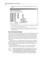
The pointer to the row is the rowid. The rowid is an Oracle-proprietary
pseudocolumn, which every row in every table has. Encrypted within it is the physical
address of the row. As rowids are not part of the SQL standard, they are never visible
to a normal SQL statement, but you can see them and use them if you want. This is
demonstrated in Figure 7-3.
The rowid for each row is globally unique. Every row in every table in the entire
database will have a different rowid. The rowid encryption provides the physical
address of the row; from which Oracle can calculate which operating system file,
and where in the file the row is, and go straight to it.
Figure 7-3 Displaying and using rowids
OCA/OCP Oracle Database 11g All-in-One Exam Guide
278
B*Tree indexes are a very efficient way of retrieving rows if the number of rows
needed is low in proportion to the total number of rows in the table, and if the table
is large. Consider this statement:
select count(*) from employees where last_name between 'A%' and 'Z%';
This WHERE clause is sufficiently broad that it will include every row in the table.
It would be much slower to search the index to find the rowids and then use the
rowids to find the rows than to scan the whole table. After all, it is the whole table
that is needed. Another example would be if the table were small enough that one
disk read could scan it in its entirety; there would be no point in reading an index first.
It is often said that if the query is going to retrieve more than two to four percent
of the rows, then a full table scan will be quicker. A special case is if the value specified
in the WHERE clause is NULL. NULLs do not go into B*Tree indexes, so a query such as
select * from employees where last_name is null;
will always result in a full table scan. There is little value in creating a B*Tree index on
a column with few unique values, as it will not be sufficiently selective: the proportion
of the table that will be retrieved for each distinct key value will be too high. In general,
B*Tree indexes should be used if
• The cardinality (the number of distinct values) in the column is high, and

• The number of rows in the table is high, and
• The column is used in WHERE clauses or JOIN conditions.
Bitmap Indexes
In many business applications, the nature of the data and the queries is such that
B*Tree indexes are not of much use. Consider the table of sales for a chain of
supermarkets, storing one year of historical data, which can be analyzed in several
dimensions. Figure 7-4 shows a simple entity-relationship diagram, with just four
of the dimensions.
Channel Sales
Date
Shop
Product
Figure 7-4
A fact table with
four dimensions
Chapter 7: DDL and Schema Objects
279
PART II
The cardinality of each dimension could be quite low. Make these assumptions:
SHOP There are four shops.
PRODUCT There are two hundred products.
DATE There are 365 days.
CHANNEL There are two channels (walk-in and delivery).
Assuming an even distribution of data, only two of the dimensions (PRODUCT
and DATE) have a selectivity that is better than the commonly used criterion of
2 percent to 4 percent, which makes an index worthwhile. But if queries use range
predicates (such as counting sales in a month, or of a class of ten or more products),
then not even these will qualify. This is a simple fact: B*Tree indexes are often useless
in a data warehouse environment. A typical query might want to compare sales
between two shops by walk-in customers of a certain class of product in a month.

There could well be B*Tree indexes on the relevant columns, but Oracle would ignore
them as being insufficiently selective. This is what bitmap indexes are designed for.
A bitmap index stores the rowids associated with each key value as a bitmap. The
bitmaps for the CHANNEL index might look like this:
WALK-IN 11010111000101011100010101
DELIVERY 00101000111010100010100010
This indicates that the first two rows were sales to walk-in customers, the third sale
was a delivery, the fourth sale was a walk-in, and so on.
The bitmaps for the SHOP index might be
LONDON 11001001001001101000010000
OXFORD 00100010010000010001001000
READING 00010000000100000100100010
GLASGOW 00000100100010000010000101
This indicates that the first two sales were in the London shop, the third was in
Oxford, the fourth in Reading, and so on. Now if this query is received:
select count(*) from sales where channel='WALK-IN' and shop='OXFORD';
Oracle can retrieve the two relevant bitmaps and add them together with a Boolean
AND operation:
WALK-IN 11010111000101011100010101
OXFORD 00100010010000010001001000
WALKIN & OXFORD 00000010000000010000001000
The result of the bitwise-AND operation shows that only the seventh and sixteenth
rows qualify for selection. This merging of bitmaps is very fast and can be used to
implement complex Boolean operations with many conditions on many columns
using any combination of AND, OR, and NOT operators. A particular advantage that
bitmap indexes have over B*Tree indexes is that they include NULLs. As far as the
bitmap index is concerned, NULL is just another distinct value, which will have its
own bitmap.
OCA/OCP Oracle Database 11g All-in-One Exam Guide
280

In general, bitmap indexes should be used if
• The cardinality (the number of distinct values) in the column is low, and
• The number of rows in the table is high, and
• The column is used in Boolean algebra operations.
TIP If you knew in advance what the queries would be, then you could build
B*Tree indexes that would work, such as a composite index on SHOP and
CHANNEL. But usually you don’t know, which is where the dynamic merging
of bitmaps gives great flexibility.
Index Type Options
There are six commonly used options that can be applied when creating indexes:
• Unique or nonunique
• Reverse key
• Compressed
• Composite
• Function based
• Ascending or descending
All these six variations apply to B*Tree indexes, but only the last three can be applied
to bitmap indexes.
A unique index will not permit duplicate values. Nonunique is the default. The
unique attribute of the index operates independently of a unique or primary key
constraint: the presence of a unique index will not permit insertion of a duplicate
value even if there is no such constraint defined. A unique or primary key constraint
can use a nonunique index; it will just happen to have no duplicate values. This is in
fact a requirement for a constraint that is deferrable, as there may be a period (before
transactions are committed) when duplicate values do exist. Constraints are discussed
in the next section.
A reverse key index is built on a version of the key column with its bytes reversed:
rather than indexing “John”, it will index “nhoJ”. When a SELECT is done, Oracle will
automatically reverse the value of the search string. This is a powerful technique for
avoiding contention in multiuser systems. For instance, if many users are concurrently

inserting rows with primary keys based on a sequentially increasing number, all their
index inserts will concentrate on the high end of the index. By reversing the keys, the
consecutive index key inserts will tend to be spread over the whole range of the index.
Even though “John” and “Jules” are close together, “nhoJ” and “seluJ” will be quite
widely separated.
A compressed index stores repeated key values only once. The default is not to
compress, meaning that if a key value is not unique, it will be stored once for each
occurrence, each having a single rowid pointer. A compressed index will store the key
once, followed by a string of all the matching rowids.
Chapter 7: DDL and Schema Objects
281
PART II
A composite index is built on the concatenation of two or more columns. There are
no restrictions on mixing datatypes. If a search string does not include all the columns,
the index can still be used—but if it does not include the leftmost column, Oracle will
have to use a skip-scanning method that is much less efficient than if the leftmost
column is included.
A function-based index is built on the result of a function applied to one or more
columns, such as upper(last_name) or to_char(startdate, 'ccyy-mm-dd').
A query will have to apply the same function to the search string, or Oracle may not
be able to use the index.
By default, an index is ascending, meaning that the keys are sorted in order of lowest
value to highest. A descending index reverses this. In fact, the difference is often not
important: the entries in an index are stored as a doubly linked list, so it is possible
to navigate up or down with equal celerity, but this will affect the order in which rows
are returned if they are retrieved with an index full scan.
Creating and Using Indexes
Indexes are created implicitly when primary key and unique constraints are defined, if
an index on the relevant column(s) does not already exist. The basic syntax for creating
an index explicitly is

CREATE [UNIQUE | BITMAP] INDEX [ schema.]indexname
ON [schema.]tablename (column [, column ] ) ;
The default type of index is a nonunique, noncompressed, non–reverse key B*Tree
index. It is not possible to create a unique bitmap index (and you wouldn’t want to if
you could—think about the cardinality issue). Indexes are schema objects, and it is
possible to create an index in one schema on a table in another, but most people
would find this somewhat confusing. A composite index is an index on several columns.
Composite indexes can be on columns of different data types, and the columns do
not have to be adjacent in the table.
TIP Many database administrators do not consider it good practice to rely on
implicit index creation. If the indexes are created explicitly, the creator has full
control over the characteristics of the index, which can make it easier for the
DBA to manage subsequently.
Consider this example of creating tables and indexes, and then defining constraints:
create table dept(deptno number,dname varchar2(10));
create table emp(empno number, surname varchar2(10),
forename varchar2(10), dob date, deptno number);
create unique index dept_i1 on dept(deptno);
create unique index emp_i1 on emp(empno);
create index emp_i2 on emp(surname,forename);
create bitmap index emp_i3 on emp(deptno);
alter table dept add constraint dept_pk primary key (deptno);
alter table emp add constraint emp_pk primary key (empno);
alter table emp add constraint emp_fk
foreign key (deptno) references dept(deptno);
OCA/OCP Oracle Database 11g All-in-One Exam Guide
282
The first two indexes created are flagged as UNIQUE, meaning that it will not be
possible to insert duplicate values. This is not defined as a constraint at this point but
is true nonetheless. The third index is not defined as UNIQUE and will therefore

accept duplicate values; this is a composite index on two columns. The fourth index
is defined as a bitmap index, because the cardinality of the column is likely to be low
in proportion to the number of rows in the table.
When the two primary key constraints are defined, Oracle will detect the preexisting
indexes and use them to enforce the constraints. Note that the index on DEPT.DEPTNO
has no purpose for performance because the table will in all likelihood be so small
that the index will never be used to retrieve rows (a scan will be quicker), but it is still
essential to have an index to enforce the primary key constraint.
Once created, indexes are used completely transparently and automatically. Before
executing a SQL statement, the Oracle server will evaluate all the possible ways of
executing it. Some of these ways may involve using whatever indexes are available;
others may not. Oracle will make use of the information it gathers on the tables and
the environment to make an intelligent decision about which (if any) indexes to use.
TIP The Oracle server should make the best decision about index use, but
if it is getting it wrong, it is possible for a programmer to embed instructions,
known as optimizer hints, in code that will force the use (or not) of certain
indexes.
Modifying and Dropping Indexes
The ALTER INDEX command cannot be used to change any of the characteristics
described in this chapter: the type (B*Tree or bitmap) of the index; the columns; or
whether it is unique or nonunique. The ALTER INDEX command lies in the database
administration domain and would typically be used to adjust the physical properties
of the index, not the logical properties that are of interest to developers. If it is necessary
to change any of these properties, the index must be dropped and recreated. Continuing
the example in the preceding section, to change the index EMP_I2 to include the
employees’ birthdays,
drop index emp_i2;
create index emp_i2 on emp(surname,forename,dob);
This composite index now includes columns with different data types. The columns
happen to be listed in the same order that they are defined in the table, but this is by

no means necessary.
When a table is dropped, all the indexes and constraints defined for the table are
dropped as well. If an index was created implicitly by creating a constraint, then dropping
the constraint will also drop the index. If the index had been created explicitly and the
constraint created later, then if the constraint were dropped the index would survive.
Exercise 7-5: Create Indexes In this exercise, add some indexes to the
CUSTOMERS table.
1. Connect to your database with SQL*Plus as user WEBSTORE.
Chapter 7: DDL and Schema Objects
283
PART II
2. Create a compound B*Tree index on the customer names and status:
create index cust_name_i on customers (customer_name, customer_status);
3. Create bitmap indexes on a low-cardinality column:
create bitmap index creditrating_i on customers(creditrating);
4. Determine the name and some other characteristics of the indexes just created
by running this query.
select index_name,column_name,index_type,uniqueness
from user_indexes natural join user_ind_columns
where table_name='CUSTOMERS';
Constraints
Table constraints are a means by which the database can enforce business rules and
guarantee that the data conforms to the entity-relationship model determined by the
systems analysis that defines the application data structures. For example, the business
analysts of your organization may have decided that every customer and every order
must be uniquely identifiable by number, that no orders can be issued to a customer
before that customer has been created, and that every order must have a valid date
and a value greater than zero. These would implemented by creating primary key
constraints on the CUSTOMER_ID column of the CUSTOMERS table and the ORDER_ID
column of the ORDERS table, a foreign key constraint on the ORDERS table referencing

the CUSTOMERS table, a not-null constraint on the DATE column of the ORDERS
table (the DATE data type will itself ensure that that any dates are valid automatically—it
will not accept invalid dates), and a check constraint on the ORDER_AMOUNT column
on the ORDERS table.
If any DML executed against a table with constraints defined violates a constraint,
then the whole statement will be rolled back automatically. Remember that a DML
statement that affects many rows might partially succeed before it hits a constraint
problem with a particular row. If the statement is part of a multistatement transaction,
then the statements that have already succeeded will remain intact but uncommitted.
EXAM TIP A constraint violation will force an automatic rollback of the
entire statement that hit the problem, not just the single action within the
statement, and not the entire transaction.
The Types of Constraint
The constraint types supported by the Oracle database are
• UNIQUE
• NOT NULL
• PRIMARY KEY
• FOREIGN KEY
• CHECK
OCA/OCP Oracle Database 11g All-in-One Exam Guide
284
Constraints have names. It is good practice to specify the names with a standard
naming convention, but if they are not explicitly named, Oracle will generate names.
Unique Constraints
A unique constraint nominates a column (or combination of columns) for which the
value must be different for every row in the table. If the constraint is based on a single
column, this is known as the key column. If the constraint is composed of more than
one column (known as a composite key unique constraint), the columns do not have to
be the same data type or be adjacent in the table definition.
An oddity of unique constraints is that it is possible to enter a NULL value into

the key column(s); it is indeed possible to have any number of rows with NULL
values in their key column(s). So selecting rows on a key column will guarantee that
only one row is returned—unless you search for NULL, in which case all the rows
where the key columns are NULL will be returned.
EXAM TIP It is possible to insert many rows with NULLs in a column with
a unique constraint. This is not possible for a column with a primary key
constraint.
Unique constraints are enforced by an index. When a unique constraint is defined,
Oracle will look for an index on the key column(s), and if one does not exist, it will
be created. Then whenever a row is inserted, Oracle will search the index to see if the
values of the key columns are already present; if they are, it will reject the insert. The
structure of these indexes (known as B*Tree indexes) does not include NULL values,
which is why many rows with NULL are permitted: they simply do not exist in the
index. While the first purpose of the index is to enforce the constraint, it has a
secondary effect: improving performance if the key columns are used in the WHERE
clauses of SQL statements. However, selecting WHERE key_column IS NULL cannot
use the index (because it doesn’t include the NULLs) and will therefore always result
in a scan of the entire table.
Not-Null Constraints
The not-null constraint forces values to be entered into the key column. Not-null
constraints are defined per column and are sometimes called mandatory columns;
if the business requirement is that a group of columns should all have values, you
cannot define one not-null constraint for the whole group but must define a not-null
constraint for each column.
Any attempt to insert a row without specifying values for the not-null-constrained
columns results in an error. It is possible to bypass the need to specify a value by
including a DEFAULT clause on the column when creating the table, as discussed in
the earlier section “Creating Tables with Column Specifications.”
Primary Key Constraints
The primary key is the means of locating a single row in a table. The relational database

paradigm includes a requirement that every table should have a primary key: a column
(or combination of columns) that can be used to distinguish every row. The Oracle
Chapter 7: DDL and Schema Objects
285
PART II
database deviates from the paradigm (as do some other RDBMS implementations)
by permitting tables without primary keys.
The implementation of a primary key constraint is in effect the union of a unique
constraint and a not-null constraint. The key columns must have unique values, and
they may not be null. As with unique constraints, an index must exist on the constrained
column(s). If one does not exist already, an index will be created when the constraint
is defined. A table can have only one primary key. Try to create a second, and you will
get an error. A table can, however, have any number of unique constraints and not-
null columns, so if there are several columns that the business analysts have decided
must be unique and populated, one of these can be designated the primary key, and
the others made unique and not null. An example could be a table of employees,
where e-mail address, social security number, and employee number should all be
required and unique.
EXAM TIP Unique and primary key constraints need an index. If one does not
exist, one will be created automatically.
Foreign Key Constraints
A foreign key constraint is defined on the child table in a parent-child relationship. The
constraint nominates a column (or columns) in the child table that corresponds to
the primary key column(s) in the parent table. The columns do not have to have the
same names, but they must be of the same data type. Foreign key constraints define
the relational structure of the database: the many-to-one relationships that connect
the table, in their third normal form.
If the parent table has unique constraints as well as (or instead of) a primary key
constraint, these columns can be used as the basis of foreign key constraints, even if
they are nullable.

EXAM TIP A foreign key constraint is defined on the child table, but a unique
or primary key constraint must already exist on the parent table.
Just as a unique constraint permits null values in the constrained column, so does
a foreign key constraint. You can insert rows into the child table with null foreign key
columns—even if there is not a row in the parent table with a null value. This creates
orphan rows and can cause dreadful confusion. As a general rule, all the columns in a
unique constraint and all the columns in a foreign key constraint are best defined
with not-null constraints as well; this will often be a business requirement.
Attempting to insert a row in the child table for which there is no matching row
in the parent table will give an error. Similarly, deleting a row in the parent table will
give an error if there are already rows referring to it in the child table. There are two
techniques for changing this behavior. First, the constraint may be created as ON
DELETE CASCADE. This means that if a row in the parent table is deleted, Oracle will
search the child table for all the matching rows and delete them too. This will happen
automatically. A less drastic technique is to create the constraint as ON DELETE SET
NULL. In this case, if a row in the parent table is deleted, Oracle will search the child