OCA /OCP Oracle Database 11g A ll-in-One Exam Guide- P37 doc

OCA/OCP Oracle Database 11g All-in-One Exam Guide
316
Data in a relational database is managed with the DML (Data Manipulation Language)
commands of SQL. These are INSERT, UPDATE, DELETE, and (with more recent
versions of SQL) MERGE. This chapter discusses what happens in memory, and on
disk, when you execute INSERT, UPDATE, or DELETE statements—the manner in
which changed data is written to blocks of table and index segments and the old
version of the data is written out to blocks of an undo segment. The theory behind
this, summarized as the ACID test, which every relational database must pass, is
explored, and you will see the practicalities of how undo data is managed.
The transaction control statements COMMIT and ROLLBACK, which are closely
associated with DML commands, are explained along with a discussion of some basic
PL/SQL objects. The chapter ends with a detailed examination of concurrent data
access and table and row locking.
Data Manipulation Language (DML) Statements
Strictly speaking, there are five DML commands:
• SELECT
• INSERT
• UPDATE
• DELETE
• MERGE
In practice, most database professionals never include SELECT as part of DML.
It is considered to be a separate language in its own right, which is not unreasonable
when you consider that the next five chapters are dedicated to describing it. The
MERGE command is often dropped as well, not because it isn’t clearly a data
manipulation command but because it doesn’t do anything that cannot be done
with other commands. MERGE can be thought of as a shortcut for executing either
an INSERT or an UPDATE or a DELETE, depending on some condition. A command
often considered with DML is TRUNCATE. This is actually a DDL (Data Definition
Language) command, but as the effect for end users is the same as for a DELETE
(though its implementation is totally different), it does fit with DML.

INSERT
Oracle stores data in the form of rows in tables. Tables are populated with rows (just as
a country is populated with people) in several ways, but the most common method is
with the INSERT statement. SQL is a set-oriented language, so any one command can
affect one row or a set of rows. It follows that one INSERT statement can insert an
individual row into one table or many rows into many tables. The basic versions
of the statement do insert just one row, but more complex variations can, with one
command, insert multiple rows into multiple tables.
Chapter 8: DML and Concurrency
317
PART II
TIP There are much faster techniques than INSERT for populating a table
with large numbers of rows. These are the SQL*Loader utility, which can
upload data from files produced by an external feeder system, and Data Pump,
which can transfer data in bulk from one Oracle database to another, either
via disk files or through a network link.
EXAM TIP An INSERT command can insert one row, with column values
specified in the command, or a set of rows created by a SELECT statement.
The simplest form of the INSERT statement inserts one row into one table, using
values provided in line as part of the command. The syntax is as follows:
INSERT INTO table [(column [,column ])] VALUES (value [,value ]);
For example:
insert into hr.regions values (10,'Great Britain');
insert into hr.regions (region_name, region_id) values ('Australasia',11);
insert into hr.regions (region_id) values (12);
insert into hr.regions values (13,null);
The first of the preceding commands provides values for both columns of the
REGIONS table. If the table had a third column, the statement would fail because it
relies upon positional notation. The statement does not say which value should be
inserted into which column; it relies on the position of the values: their ordering in

the command. When the database receives a statement using positional notation, it
will match the order of the values to the order in which the columns of the table are
defined. The statement would also fail if the column order was wrong: the database
would attempt the insertion but would fail because of data type mismatches.
The second command nominates the columns to be populated and the values
with which to populate them. Note that the order in which columns are mentioned
now becomes irrelevant—as long as the order of the columns is the same as the order
of the values.
The third example lists one column, and therefore only one value. All other
columns will be left null. This statement will fail if the REGION_NAME column is
not nullable. The fourth example will produce the same result, but because there
is no column list, some value (even a NULL) must be provided for each column.
TIP It is often considered good practice not to rely on positional notation
and instead always to list the columns. This is more work but makes the code
self-documenting (always a good idea!) and also makes the code more resilient
against table structure changes. For instance, if a column is added to a table, all
the INSERT statements that rely on positional notation will fail until they are
rewritten to include a NULL for the new column. INSERT code that names
the columns will continue to run.
OCA/OCP Oracle Database 11g All-in-One Exam Guide
318
To insert many rows with one INSERT command, the values for the rows must
come from a query. The syntax is as follows:
INSERT INTO table [column [, column ] ] subquery;
Note that this syntax does not use the VALUES keyword. If the column list is
omitted, then the subquery must provide values for every column in the table. To
copy every row from one table to another, if the tables have the same column
structure, a command such as this is all that is needed:
insert into regions_copy select * from regions;
This presupposes that the table REGIONS_COPY does exist. The SELECT subquery

reads every row from the source table, which is REGIONS, and the INSERT inserts
them into the target table, which is REGIONS_COPY.
EXAM TIP Any SELECT statement, specified as a subquery, can be used as
the source of rows passed to an INSERT. This enables insertion of many rows.
Alternatively, using the VALUES clause will insert one row. The values can be
literals or prompted for as substitution variables.
To conclude the description of the INSERT command, it should be mentioned
that it is possible to insert rows into several tables with one statement. This is not
part of the OCP examination, but for completeness here is an example:
insert all
when 1=1 then
into emp_no_name (department_id,job_id,salary,commission_pct,hire_date)
values (department_id,job_id,salary,commission_pct,hire_date)
when department_id <> 80 then
into emp_non_sales (employee_id,department_id,salary,hire_date)
values (employee_id,department_id,salary,hire_date)
when department_id = 80 then
into emp_sales (employee_id,salary,commission_pct,hire_date)
values (employee_id,salary,commission_pct,hire_date)
select employee_id,department_id,job_id,salary,commission_pct,hire_date
from employees where hire_date > sysdate - 30;
To read this statement, start at the bottom. The subquery retrieves all employees
recruited in the last 30 days. Then go to the top. The ALL keyword means that every
row selected will be considered for insertion into all the tables following, not just into
the first table for which the condition applies. The first condition is 1=1, which is
always true, so every source row will create a row in EMP_NO_NAME. This is a copy
of the EMPLOYEES table with the personal identifiers removed. The second condition
is DEPARTMENT_ID <> 80, which will generate a row in EMP_NON_SALES for every
employee who is not in the sales department; there is no need for this table to have
the COMMISSION_PCT column. The third condition generates a row in EMP_SALES

Chapter 8: DML and Concurrency
319
PART II
for all the salesmen; there is no need for the DEPARTMENT_ID column, because they
will all be in department 80.
This is a simple example of a multitable insert, but it should be apparent that with
one statement, and therefore only one pass through the source data, it is possible to
populate many target tables. This can take an enormous amount of strain off the
database.
Exercise 8-1: Use the INSERT Command In this exercise, use various
techniques to insert rows into a table.
1. Connect to the WEBSTORE schema with either SQL Developer or SQL*Plus.
2. Query the PRODUCTS, ORDERS, and ORDER_ITEMS tables, to confirm what
data is currently stored:
select * from products;
select * from orders;
select * from order_items;
3. Insert two rows into the PRODUCTS table, providing the values in line:
insert into products values (prod_seq.nextval, '11G SQL Exam Guide',
'ACTIVE',60,sysdate, 20);
insert into products
values (prod_seq.nextval, '11G All-in-One Guide',
'ACTIVE',100,sysdate, 40);
4. Insert two rows into the ORDERS table, explicitly providing the column
names:
insert into orders (order_id, order_date, order_status, order_amount, customer_id)
values (order_seq.nextval, sysdate, 'COMPLETE', 3, 2);
insert into orders (order_id, order_date, order_status, order_amount, customer_id)
values (order_seq.nextval, sysdate, 'PENDING', 5, 3);
5. Insert three rows into the ORDER_ITEMS table, using substitution variables:

insert into order_items values (&item_id, &order_id, &product_id, &quantity);
When prompted, provide the values: {1, 1, 2,5}, {2,1,1,3}, and {1,2,2,4}.
6. Insert a row into the PRODUCTS table, calculating the PRODUCT_ID to be
100 higher than the current high value. This will need a scalar subquery:
insert into products values ((select max(product_id)+100 from products),
'11G DBA2 Exam Guide', 'INACTIVE', 40, sysdate-365, 0);
7. Confirm the insertion of the rows:
select * from products;
select * from orders;
select * from order_items;
8. Commit the insertions:
commit;
OCA/OCP Oracle Database 11g All-in-One Exam Guide
320
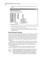
The following illustration shows the results of the exercise, using SQL*Plus:
UPDATE
The UPDATE command is used to change rows that already exist—rows that have
been created by an INSERT command, or possibly by a tool such as Data Pump. As
with any other SQL command, an UPDATE can affect one row or a set of rows. The
size of the set affected by an UPDATE is determined by a WHERE clause, in exactly the
same way that the set of rows retrieved by a SELECT statement is defined by a WHERE
clause. The syntax is identical. All the rows updated will be in one table; it is not
possible for a single update command to affect rows in multiple tables.
When updating a row or a set of rows, the UPDATE command specifies which
columns of the row(s) to update. It is not necessary (or indeed common) to update
every column of the row. If the column being updated already has a value, then this
value is replaced with the new value specified by the UPDATE command. If the
column was not previously populated—which is to say, its value was NULL—then
it will be populated after the UPDATE with the new value.
A typical use of UPDATE is to retrieve one row and update one or more columns

of the row. The retrieval will be done using a WHERE clause that selects a row by its
primary key, the unique identifier that will ensure that only one row is retrieved. Then
the columns that are updated will be any columns other than the primary key column.
It is very unusual to change the value of the primary key. The lifetime of a row begins
when it is inserted, then may continue through several updates, until it is deleted.
Throughout this lifetime, it will not usually change its primary key.
To update a set of rows, use a less restrictive WHERE clause than the primary key.
To update every row in a table, do not use any WHERE clause at all. This set behavior
can be disconcerting when it happens by accident. If you select the rows to be updated
with any column other than the primary key, you may update several rows, not just one.
If you omit the WHERE clause completely, you will update the whole table—perhaps
millions of rows updated with just one statement—when you meant to change just one.
Chapter 8: DML and Concurrency
321
PART II
EXAM TIP One UPDATE statement can change rows in only one table, but it
can change any number of rows in that table.
An UPDATE command must honor any constraints defined for the table, just
as the original INSERT would have. For example, it will not be possible to update a
column that has been marked as mandatory to a NULL value or to update a primary
key column so that it will no longer be unique. The basic syntax is the following:
UPDATE table SET column=value [,column=value ] [WHERE condition];
The more complex form of the command uses subqueries for one or more of the
column values and for the WHERE condition. Figure 8-1 shows updates of varying
complexity, executed from SQL*Plus.
The first example is the simplest. One column of one row is set to a literal value.
Because the row is chosen with a WHERE clause that uses the equality predicate on
the table’s primary key, there is an absolute guarantee that at most only one row will
be affected. No row will be changed if the WHERE clause fails to find any rows at all.
The second example shows use of arithmetic and an existing column to set the new

value, and the row selection is not done on the primary key column. If the selection is
not done on the primary key, or if a nonequality predicate (such as BETWEEN) is used,
then the number of rows updated may be more than one. If the WHERE clause is
omitted entirely, the update will be applied to every row in the table.
The third example in Figure 8-1 introduces the use of a subquery to define the set
of rows to be updated. A minor additional complication is the use of a replacement
variable to prompt the user for a value to use in the WHERE clause of the subquery.
Figure 8-1 Examples of using the UPDATE statement
OCA/OCP Oracle Database 11g All-in-One Exam Guide
32 2
In this example, the subquery (lines 3 and 4) will select every employee who is in a
department whose name includes the string ‘IT’ and increment their current salary
by 10 percent (unlikely to happen in practice).
It is also possible to use subqueries to determine the value to which a column will
be set, as in the fourth example. In this case, one employee (identified by primary key,
in line 5) is transferred to department 80 (the sales department), and then the subquery
in lines 3 and 4 sets his commission rate to whatever the lowest commission rate in
the department happens to be.
The syntax of an update that uses subqueries is as follows:
UPDATE table
SET column=[subquery] [,column=subquery ]
WHERE column = (subquery) [AND column=subquery ] ;
There is a rigid restriction on the subqueries using update columns in the SET
clause: the subquery must return a scalar value. A scalar value is a single value of
whatever data type is needed: the query must return one row, with one column. If
the query returns several values, the UPDATE will fail. Consider these two examples:
update employees
set salary=(select salary from employees where employee_id=206);
update employees
set salary=(select salary from employees where last_name='Abel');

The first example, using an equality predicate on the primary key, will always
succeed. Even if the subquery does not retrieve a row (as would be the case if there
were no employee with EMPLOYEE_ID equal to 206), the query will still return a
scalar value: a null. In that case, all the rows in EMPLOYEES would have their SALARY
set to NULL—which might not be desired but is not an error as far as SQL is concerned.
The second example uses an equality predicate on the LAST_NAME, which is not
guaranteed to be unique. The statement will succeed if there is only one employee
with that name, but if there were more than one it would fail with the error
“ORA-01427: single-row subquery returns more than one row.” For code that will
work reliably, no matter what the state of the data, it is vital to ensure that the
subqueries used for setting column values are scalar.
TIP A common fix for making sure that queries are scalar is to use MAX or
MIN. This version of the statement will always succeed:
update employees
set salary=(select max(salary) from employees where
last_name='Abel');
However, just because it will work, doesn’t necessarily mean that it does what
is wanted.
The subqueries in the WHERE clause must also be scalar, if it is using the equality
predicate (as in the preceding examples) or the greater/less than predicates. If it is
using the IN predicate, then the query can return multiple rows, as in this example
which uses IN:
Chapter 8: DML and Concurrency
323
PART II
update employees
set salary=10000
where department_id in (select department_id from departments
where department_name like '%IT%');
This will apply the update to all employees in a department whose name includes

the string ‘IT’. There are several of these. But even though the query can return several
rows, it must still return only one column.
EXAM TIP The subqueries used to SET column values must be scalar
subqueries. The subqueries used to select the rows must also be scalar,
unless they use the IN predicate.
Exercise 8-2: Use the UPDATE Command In this exercise, use various
techniques to update rows in a table. It is assumed that the WEBSTORE.PRODUCTS
table is as seen in the illustration at the end of Exercise 8-1. If not, adjust the values
as necessary.
1. Connect to the WEBSTORE schema using SQL Developer or SQL*Plus.
2. Update a single row, identified by primary key:
update products set product_description='DBA1 Exam Guide'
where product_id=102;
This statement should return the message “1 row updated.”
3. Update a set of rows, using a subquery to select the rows and to provide values:
update products
set product_id=(1+(select max(product_id) from products where product_id <> 102))
where product_id=102;
This statement should return the message “1 row updated.”
4. Confirm the state of the rows:
select * from products;
5. Commit the changes made:
commit;
DELETE
Previously inserted rows can be removed from a table with the DELETE command.
The command will remove one row or a set of rows from the table, depending on a
WHERE clause. If there is no WHERE clause, every row in the table will be removed
(which can be a little disconcerting if you left out the WHERE clause by mistake).
TIP There are no “warning” prompts for any SQL commands. If you instruct
the database to delete a million rows, it will do so. Immediately. There is none

of that “Are you sure?” business that some environments offer.
OCA/OCP Oracle Database 11g All-in-One Exam Guide
324
A deletion is all or nothing. It is not possible to nominate columns. When rows
are inserted, you can choose which columns to populate. When rows are updated, you
can choose which columns to update. But a deletion applies to the whole row—the
only choice is which rows in which table. This makes the DELETE command syntactically
simpler than the other DML commands. The syntax is as follows:
DELETE FROM table [WHERE condition];
This is the simplest of the DML commands, particularly if the condition is omitted.
In that case, every row in the table will be removed with no prompt. The only
complication is in the condition. This can be a simple match of a column to a literal:
delete from employees where employee_id=206;
delete from employees where last_name like 'S%';
delete from employees where department_id=&Which_department;
delete from employees where department_id is null;
The first statement identifies a row by primary key. One row only will be
removed—or no row at all, if the value given does not find a match. The second
statement uses a nonequality predicate that could result in the deletion of many
rows: every employee whose surname begins with an uppercase “S.” The third
statement uses an equality predicate but not on the primary key. It prompts for
a department number with a substitution variable, and all employees in that
department will go. The final statement removes all employees who are not
currently assigned to a department.
The condition can also be a subquery:
delete from employees where department_id in
(select department_id from departments where location_id in
(select location_id from locations where country_id in
(select country_id from countries where region_id in
(select region_id from regions where region_name='Europe')

)
)
)
This example uses a subquery for row selection that navigates the HR geographical
tree (with more subqueries) to delete every employee who works for any department
that is based in Europe. The same rule for the number of values returned by the
subquery applies as for an UPDATE command: if the row selection is based on an
equality predicate (as in the preceding example) the subquery must be scalar, but if
it uses IN the subquery can return several rows.
If the DELETE command finds no rows to delete, this is not an error. The
command will return the message “0 rows deleted” rather than an error message
because the statement did complete successfully—it just didn’t find anything to do.
Exercise 8-3: Use the DELETE Command In this exercise, use various
techniques to delete rows in a table. It is assumed that the WEBSTORE.PRODUCTS
table has been modified during the previous two exercises. If not, adjust the values
as necessary.
Chapter 8: DML and Concurrency
325
PART II
1. Connect to the WEBSTORE schema using SQL Developer or SQL*Plus.
2. Remove one row, using the equality predicate on the primary key:
delete from products where product_id=3;
This should return the message “1 row deleted.”
3. Attempt to remove every row in the table by omitting a WHERE clause:
delete from products;
This will fail, due to a constraint violation because there are child records
in the ORDER_ITEMS table that reference PRODUCT_ID values in the
PRODUCTS table via the foreign key constraint FK_PRODUCT_ID.
4. Commit the deletion:
commit;

To remove rows from a table, there are two options: the DELETE command and
the TRUNCATE command. DELETE is less drastic, in that a deletion can be rolled
back whereas a truncation cannot be. DELETE is also more controllable, in that it is
possible to choose which rows to delete, whereas a truncation always affects the whole
table. DELETE is, however, a lot slower and can place a lot of strain on the database.
TRUNCATE is virtually instantaneous and effortless.
TRUNCATE
The TRUNCATE command is not a DML command; it is a DDL command. The
difference is enormous. When DML commands affect data, they insert, update, and
delete rows as part of transactions. Transactions are defined later in this chapter, in
the section “Control Transactions.” For now, let it be said that a transaction can be
controlled, in the sense that the user has the choice of whether to make the work
done in a transaction permanent, or whether to reverse it. This is very useful but
forces the database to do additional work behind the scenes that the user is not aware
of. DDL commands are not user transactions (though within the database, they are in
fact implemented as transactions—but developers cannot control them), and there is
no choice about whether to make them permanent or to reverse them. Once executed,
they are done. However, in comparison to DML, they are very fast.
EXAM TIP Transactions, consisting of INSERT, UPDATE, and DELETE (or even
MERGE) commands, can be made permanent (with a COMMIT) or reversed
(with a ROLLBACK). A TRUNCATE command, like any other DDL command,
is immediately permanent: it can never be reversed.
From the user’s point of view, a truncation of a table is equivalent to executing a
DELETE of every row: a DELETE command without a WHERE clause. But whereas
a deletion may take some time (possibly hours, if there are many rows in the table), a
truncation will go through instantly. It makes no difference whether the table contains
one row or billions; a TRUNCATE will be virtually instantaneous. The table will still
exist, but it will be empty.