Stephens & Foraging - Behavior and Ecology - Chapter 9 docx
Bạn đang xem bản rút gọn của tài liệu. Xem và tải ngay bản đầy đủ của tài liệu tại đây (212.54 KB, 26 trang )
9
Foraging in the Face of Danger
Peter A. Bednekoff
9.1 Prologue
A juvenile coho salmon holds its position in the flow of a brook. To
conserve energy, it positions itself in the lee of a small rock. Distinc-
tive blotches of color on its sides, called parr marks, provide effective
camouflage. As long as it holds its position, it is virtually impossible to
see. The simple strategy of keeping still hides it from the prying eyes of
potential salmon-eaters. Kingfishers and herons threaten from above,
and cutthroat trout, permanent residents of the stream, seldom reject a
meal of young salmon. The threat posed by these and other predators
is ever present.
The clear water flowing past the salmon presents a stream of food
items: midges struggle on the surface; mayfly nymphs drift in the cur-
rent. But, here’s the rub: to capture a prey item, the salmon must dash
out from its station, potentially telegraphing its position to unwelcome
observers. When the salmon feels safe, it will travel quite a distance to
intercept a food item, making a leisurely excursion to collect a drifting
midge as far as a meter away from its location.
Detecting a predator changes the salmon’s behavior. Depending on
the level of the perceived threat, the salmon has several options. It may
flush to deep water or another safe location. It may stop feeding alto-
gether, but hold its position. It may continue feeding, but dramatically
306 Peter A. Bednekoff
Figure 9.1. Patch residence time increases with travel time between patches (as predicted), but blue jays
stay in patches much longer than the optimal residence time. Solid squares show observed residence
times; open squares show the predicted optimal residence times. (After Kamil et al. 1993.)
reduce the distance it will travel to intercept food. This series of graded re-
sponses represents a sophisticated and often effective strategy to avoid preda-
tors. Sophisticated or not, all of these responses reduce the salmon’s feeding
efficiency. The salmon’s problem is far from unique; virtually all animals face
a trade-off between acquiring resources and becoming a resource for another.
9.2 Overview and Road Map
Resource acquisition is necessary for fitness, but it is not sufficient. Food is
generally good for the forager, but not if the forager is dead. Danger affects
animal decisions in many ways (see reviews in Lima and Dill 1990; Lima
1998). Animals often face a trade-off between food acquisition and danger:
the alternative that yields the highest rates of food intake is also the most
dangerous. A growing area of research focuses on this fundamental trade-off.
This chapter examines how danger from predators affects foraging behavior.
Early theory assumed that fitness was highest when the net rate of foraging
gain (i.e., net amount of energy acquired per unit time) was highest. Early
empirical tests consistently showed that foragers are sensitive to foraging gain
(see Stephens and Krebs 1986). As predicted, many animals spend more time
feeding in each patch when patches are farther apart (Stephens and Krebs
1986; Nonacs 2001). Animals often stay in patches longer, however, than
the time that would maximize their overall rate of energy gain (Kamil et al.
1993; Nonacs 2001; fig. 9.1). Tests suggested that early rate-maximizing
models were partly right: foragers are sensitive to their rate of energy gain,
but often do not fully maximize it (see also Nonacs 2001). This observation
Foraging in the Face of Danger 307
Distance from cover (m)
% carried to cover
0
20
40
0
5
10
60
80
100
15
20
after hawk scare
before hawk scare
Figure 9.2. Black-capped chickadees are more likely to carry small food items to cover before eating
them when cover is close and after a simulated hawk attack. (After Lima 1985a.)
suggested that some non-energetic costs must be important. By pointing out
the importance of such costs, early tests of rate-maximizing models provided
the springboard for the study of foraging and danger.
Black-capped chickadees often carry food items from a feeder to a bush
before consuming them. They are more likely to carry larger items and are
more likely to carry items if the feeder is closer to a bush (Lima 1985a; fig.
9.2). Carrying an item to a bush decreases a chickadee’s rate of intake, but
intake rate is decreased less with large items and close distances. Steve Lima
hypothesized that chickadees carried food to cover in order to reduce their
exposure to predators. He tested this hypothesis by flying a hawk model in
the area during some trials. After having seen the hawk model, chickadees
were more likely to carry food to safety (Lima 1985a; fig. 9.2). Thus, animals
are willing to reduce their intake rate in order to reduce danger.
To begin this chapter, I examine why foraging gain and danger are gen-
erally linked, and I build a life history framework for modeling foraging and
danger. I discuss how danger may change with the internal state of the ani-
mal, time, and group size. These topics lead to inquiries on how animals assess
danger and whether they should overestimate danger. I close with my view
of the prospects of the field. Within each section, I outline some principles,
often with the help of simple models, and illustrate those principles with a
sampling of examples.
9.3 Why Does Increased Foraging Lead to Greater Danger?
Animals often face alternatives that differ in both foraging gain and danger.
Obviously, foragers should avoid options that combine poor feeding with
308 Peter A. Bednekoff
great danger and choose options that offer good feeding with little danger.
Most often, however, animals face difficult choices in which the options for
better feeding also entail greater danger. Such difficult choices are ubiquitous
for several reasons, and wherever one or more of these reasons applies, organ-
isms face a trade-off between feeding and danger. After sketching out various
routes to a trade-off, I return to a general conceptual approach because the
many routes to a trade-off converge on the same basic consequences.
Time Spent Exposed
Guppies feed day and night when no predators are around, but only during
the day if predators are around (Fraser et al. 2004). In response to indications
of danger, many animals restrict their feeding time (Lima 1998, see especially
table II). An animal that feeds part of the time can restrict its feeding to the
safest period, but it must extend its feeding time into more dangerous periods
in order to feed for longer. For example, small birds must extend their feeding
time into the twilight periods around dusk and dawn, when they are less able
to detect attacks in the low light and deep shadows (see Lima 1988a, 1988c;
Krams 2000). For bats that feed on insects, darkness is safer, but emerging
before nightfall may allow greater feeding ( Jones and Rydell 1994). Feeding
at nightisalso saferfor minnows (Greenwoodand Metcalfe 1998)and juvenile
salmon (Metcalfe et al. 1999). In order to increase feeding, however, these
fish have to feed during the more dangerous daylight period.
Habitat Choice
While actively foraging, animals often choose between habitats that differ in
danger and productivity. For example, aquatic snails feeding on algae face a
trade-off because more algae grows on the sunny side of rocks, but the tops
of rocksarealso moreexposed tofish predators (Levri1998). Thebasic ecology
of exposure leads to the trade-off: exposure to sunlight allows more photo-
synthesis, but exposure often leaves foragers more vulnerable to predators.
Similarly, sunfish can find more zooplankton to eat in the open-water por-
tions oflakes because theseareas produce morephytoplankton, which support
the zooplankton. The open areas, however, provide no refuge from attack,
whereas the weedy littoral zone provides refuge, but less food (Werner and
Hall 1988). Animals switch between these two kinds of areas during growth
because both foraging gain and danger change as they grow (Werner and Gil-
liam 1984).
In other cases, the attack strategy of the predator and the escape strategy
of the prey combine to create the trade-off. In boreal forests, the swooping
Foraging in the Face of Danger 309
attacks of pygmy owls make the outer, lower branches of trees particularly
dangerous (Kullberg 1995), and small birds avoid these branches unless com-
petition or hunger forces them there (e.g., Krams 1996; Kullberg 1998b).
Within a foraging group, individuals on the leading edge will first encounter
new sources of both food and danger (Bumann et al. 1997). Animals often
move to edge positions when hungry (Romey 1995) and to central positions
when alarmed (Krause 1993). Habitat choice may involve another layer of
compromise when foragers face conflicting pressures from different kinds of
predators. For example, grasshoppers can reduce bird predation by staying
low on a blade of grass, but they can minimize predation by lizards and small
mammals by positioning themselves high on grass stems. When both kinds of
predators are around, grasshoppers choose intermediate positions (Pitt 1999).
As theseexamples emphasize,animals choosebetween habitatson small aswell
as large spatial scales, and both kinds of choices have ecological consequences.
Movement
Creatures great and small move less when predators are around (Lima 1998,
table II). A forager actively searching for food can cover a greater area by
movingfaster. Bycovering a greaterarea, itislikely toencountermore feeding
opportunities, and may also encounter more predators (Werner and Anholt
1993). Besides simply crossing paths with more predators, moving foragers
increase the likelihood of an attack. Anaesthetized tadpoles are less likely to be
killed by aquatic invertebrate predators (Skelly 1994), and tadpoles generally
move less when danger is greater (Anholt et al. 2000). When movement is in
short bursts, as in degus, greater movement may involve both faster speeds
while moving and shorter pauses between bursts (Vasquez et al. 2002). I will
consider movement in further detail below after developing a general model
of foraging in the face of danger.
Detection Behavior
Most animals perform behaviors that increase their chances of detecting and
escaping from predators. The best studied of these behaviors are pauses dur-
ing foraging to scan the environment for potential danger (see Bednekoff and
Lima 1998a; Treves 2000). Animals can raise their rate of food consumption
by scanning less frequently, but at the cost of detecting attacks less effectively
(e.g., Wahungu et al. 2001). Investigators have often operationally defined
vigilance as raising the head above horizontal. While this operational defini-
tion works well for birds and mammals, animals with different body forms
and lifestyles may require other operational definitions. For example, lizards
310 Peter A. Bednekoff
basking with their eyes shut and one or more limbs raised off the substratum
seem to be showing little antipredator behavior (Downes and Hoefer 2004).
Overall, the varied postures and attention required for foraging probably
affect predator detection in many organisms. For example, guppies react less
quickly to predators when foraging than when not foraging, and even less
quickly when foraging nose down (Krause and Godin 1996).
Depletion and Density Dependence
For a burrowing animal such as a marmot, safety comes from fleeing back to
the burrow (Holmes 1984; Blumstein 1998). Marmots feed near their bur-
rows, and so deplete food in the area (Del Moral 1984). Due to this depletion,
a marmot can feed at a higher rate, but at greater danger, by venturing farther
from the burrow. Thus, reactions to initial differences in danger produce dif-
ferences in foraging. Many lizards also feed from a safe central place (Cooper
2000). Such lizards can find more prey farther out, but at a cost. The actions
of a lizard also produce a gradient of food and danger for its potential prey.
The grasshoppers the lizard preys on can find a richer, less depleted food
supply near the lizard’s perch, but obviously, feeding near the lizard increases
the possibility of attack (Chase 1998). Thus, a spatial trade-off at one trophic
level may have cascading effects on other trophic levels.
In a manner similar to food depletion, density dependence can produce a
trade-off whenpotential preycongregate. By congregating,prey decreaseone
another’s feeding rates through competition and also decrease one another’s
danger through safety-in-numbers advantages. When avoiding predatory
perch, 92% of small crucian carp concentrate in the safer shallows, compoun-
ding the differences in food availability between shallows and open waters
(Paszkowski et al. 1996). In theory, the outcome depends on the balance of
competitive and safety-in-numbers effects and on how free predators are to
choose habitats, but we may often expect habitats to be made either safe but
poor orrich butdangerous bythese mechanisms(Hugie and Dill 1994; Moody
et al. 1996; Sih 1998).
9.4 Modeling Foraging under Danger of Predation
Foraging for a Fixed Time
Bluehead chubs alter their foraging in response to changes in energetic returns
and danger from green sunfish. The best explanation for their behavior com-
bines food and danger in a life history context (Skalski and Gilliam 2002). To
build models of foraging under danger of predation, we start from the first
Foraging in the Face of Danger 311
principle of foraging theory—that food is good. We assume that higher for-
aging success leads to greater reproductive success in the future. To include
danger, we need a second principle—that death is bad for fitness. Early re-
search was uncertain on how to incorporate danger into foraging models (see
box 1.1), perhaps because it is not obvious how to combine the benefits of
foraging and the costs of predation. Because the costs and benefits are in
different units, we need to translate both foraging gain and danger into some
measure of fitness. A life history perspective isessential, and it leads to a simple
solution that exists precisely because the costs and benefits of foraging under
danger of predation are linked.
Decisions made under danger of predation are life history problems be-
cause, if predation occurs, the forager’s life is history. In a life history, the
basic currency to maximize is expected reproductive value, b + SV, where
b is current reproduction, S is survival to the following breeding season, and
V is the expected reproductive value for an animal that does survive to the
next breeding season (see Stearns 1992). I concentrate here on foraging and
fitness during a period without current reproduction (b = 0), so the measure
of fitness is SV, the future benefits multiplied by the odds of surviving to
realize them. I expect increased foraging to decrease survival to the time of
reproduction, but to increase future reproduction if the animal does survive.
Death lowers expected future fitness to zero. Therefore, the cost of being
killed is the reproductive success a forager could have had if it had survived.
This linkage means that when we ask how much risk a forager should accept
to produce one additional offspring, we need to know how many offspring it
would produce otherwise. For example, a forager that would otherwise ex-
pect to produce one offspring might risk a lot to produce a second, while a
forager that would otherwise expect to produce three offspring should risk
less to produce a fourth,and a forager that would otherwise expect to produce
a dozen should risk little to produce a thirteenth. This linkage of costs and
benefits sets up an automatic state dependence: the potential losses from being
killed increase with previous foraging success, so the relative value of further
foraging is likely to be lower (see Clark 1994). Even if the fitness gains of
foraging are constant, the costs should increase, since the expected reproduc-
tive value increases, and that entire value would be lost in death. In line with
this logic, juvenile coho salmon are more cautious when they are larger, be-
cause larger individuals expect greater reproduction if they survive to breed
(Reinhardt and Healey 1999).
Now I will repeat these arguments mathematically. For a nonreproducing
animal, fitness equals the future value of foraging discounted by the probabil-
ity of surviving from now until then, W(u) =S(u)V(u), where uis a measure of
foraging effort, W is fitness, S is survival, and V is future reproductive value.
312 Peter A. Bednekoff
Fitness, survival, and future reproductive value are all functions of foraging
effort u. In general, we expect survival to decrease and future reproductive value
toincrease withforagingeffort. Morespecifically,we expectsurvivalto decre-
ase exponentially with mortality, S(u) =exp[−M(u)], where M(u) is mortality.
Mortality rate, M(u), and future reproductive value, V(u), could take var-
ious mathematical forms. For simplicity, I define foraging effort as a fraction
of the maximum possible effort, so that u varies from zero to one and does
not have units. This allows mortality, M(u), and future reproduction, V(u),
to be given as simple functions of foraging effort.
Mortality is a function of the amount of time spent exposed to attack,
the attack rate per unit time, and the probability of dying when attacked
(see Lima and Dill 1990). Greater overall foraging effort could affect any of
these components. For now I use a descriptive equation for mortality, M(u)
=ku
z
, where k is a constant and the exponent z gives the overall shape of the
trade-off. Later we will examine two specific cases to see what k and z might
mean biologically, but for now I will simply label k as the mortality constant
and z as themortality exponent. The general principle is that mortality should
increase with foraging effort at a linear or accelerating rate; that is, M(u) =
ku
z
with z ≥ 1. If foragers exercise their safest options first, we expect
an accelerating function because additional food comes from increasingly
dangerous options. A mathematically convenient value for the exponent, z =
2, matches observed changes in behavior well enough (Werner and Anholt
1993), but othervalues are notruled out, so Ialso examine alinear relationship
(z = 1) as well as more sharply accelerating ones (z = 3andz = 4). For all
values, survival declines as foraging effort increases, but the contours of the
decline depend on the exponent of the mortality function, z (fig. 9.3). As we
Figure 9.3. Survival declines with foraging effort. The swiftness of the decline varies with z, the exponent
of the curve relating foraging effort to mortality.
Foraging in the Face of Danger 313
shall see near the end of this chapter, the value of this exponent determines
whether foragers should over- or underestimate danger.
For therelationship betweenforaging effortand future reproductive value,
we will useV(u) =κu. Inthisequation, theconstant κ translates foragingeffort
into future offspring, and u is foraging effort. We expect future reproductive
value to increase with total foraging effort. Studies have shown that greater
foraging success leads to greater fitness in adult crab spiders (Morse and
Stephens 1996), water striders (Blanckenhorn 1991), and water pipits (Frey-
Roos etal. 1995).Particularly forany organismsthat areable togrow, reduced
foraging in the presence of predators can lead to considerable long-term losses
of potential reproduction (Martin and Lopez 1999; see also Lima 1998, table
III).
Alinear relationshipbetweenforaging andfuturereproductive valueisuse-
ful forits simplicity.Other relationshipsmay occurin nature,and therelation-
ship may differ between the sexes even within a species (Merilaita and Jor-
malainen 2000). I use alinear relationship here because it allows simplemodels
with clear conclusions, even though these models may somewhat understate
the effects of danger. The results of more complex models, in which future
fitness is a decelerating function of foraging gain, strongly support the con-
clusions I reach using this simpler linear relationship.
To complete the modeling framework, assume that foraging effort must
be greater than some required effort, R. This requirement, R,istherequired
rate of feeding divided by the maximum rate of feeding and so is a proportion
without units. A forager starves if its foraging effort is less than the require-
ment, and avoids starvation as long as its foraging effort is greater than the
requirement. A forager gains some amount of fitness, V(R), by just meeting
the requirement, but increases its future reproductive value by foraging at a
rate higher than the requirement.
Assembling the pieces described above, we get the overall equation for
fitness: W(u) =S(u)V(u) =[exp(−ku
z
)][κu]. We can find the optimal foraging
effort, u
∗
, if we differentiate W(u), set the derivative to zero, and solve for u.
We find that
u
∗
=
1
z
√
kz
, (9.1)
so long as u
∗
≥ R.
The foraging effort that maximizes fitness (i.e., is optimal) decreases as the
danger constant k increases. As the mortality exponent z increases, optimal
foraging effort decreases less sharply with increases in k (fig. 9.4). Modelers
sometimes assume that animals maximize survival during the nonbreeding
season (see McNamara and Houston 1982, 1986; Houston and McNamara
314 Peter A. Bednekoff
Figure 9.4. Optimal foraging effort declines with the expected number of attacks by predators. The swift-
ness of the decline varies with z, the exponent of the curve relating foraging effort to mortality.
1999). This assumption is justified whenever the requirement is greater than
the feeding rate that would otherwise be optimal, R > 1/(
z
√
kz) . Thus, a life
history approach can converge on models that assume survival maximization
even when future reproductive value increases linearly with foraging effort.
In order to examine our model further, we need to look more closely
at the relationship between mortality and foraging effort, m(u) = ku
z
.Mor-
tality depends on the encounter rate with predators, time spent exposed to
predators, and the probability of being killed per encounter. The relationship
between mortality and foraging effort includes effects on any of these three
components. I consider two situations here.
First, considertadpoles encountering predatorydragonfly larvae.Tadpoles
move while foraging, while dragonfly larvae sit and wait for prey. If a tadpole
moves faster, it encounters both more food and more predators. In this case,
the exponent, z, reflects changes in metabolic cost per distance moved and
the constant, k, combines the relative encounter rate with predators and the
probability of being killed in an encounter. This logic applies to any forager
moving at different speeds with relatively immobile food and predators.
Second, consider birds hunted by Accipiter hawks, which move a great
deal while hunting. Because the hawks seek them out, greater foraging effort
will not cause foragers to encounter more predators, but it may make them
more likely to be killed when they do encounter a predator. In this case, the
constant k includes a constant attack rate, α, and the exponent, z, reflects
how foraging effort increases the probability of being killed in an attack. This
logic applies when predators move rapidly and foragers are relatively im-
mobile.
Foraging in the Face of Danger 315
The interpretation of the mortality function, m(u) = ku
z
, depends on the
biology of the predators and prey. I use the second scenario to gain some in-
sight into models that maximize survival. Here an animal is exposed for a
period T at an attack rate α. Thus, αT is the number of attacks the animal
can expect while foraging. The optimal feeding rate will approach the re-
quirement with only a modest number of attacks at a moderate level of re-
quirement, particularly if the mortality exponent z is small (see fig. 9.4), and
will approach any level of requirement if the expected number of attacks is
large enough. Danger can cause animals to behave as if they are foraging to
meet a set requirement.
Gathering Resources with No Time Limit
So far, we have considered foraging for a fixed time. We can modify our
framework to address the classic problem of gaining a fixed amount of re-
sources from foraging within a potentially unlimited amount of time (Gilliam
1982; see also Werner and Gilliam 1984; Stephens and Krebs 1986; Houston
et al. 1993). Here a fixed amount of reproduction, V, occurs whenever suf-
ficient resources, K, are accumulated. Thus, the reproductive value is fixed,
but the time to reach it depends on gain, so W(u) = exp[−M(u)T(u)]V,and
T(u) = K/u − R. In this function, fitness will be maximized when M(u)/
(u − R) is minimized, which is another rendering of Gilliam’s M/g rule (see
box 1.1). Using our equation for mortality, M(u) = ku
z
, we differentiate and
solve for the optimal foraging effort,
u
∗
=
zR
z − 1
(9.2)
The mortality exponent, z, is the key parameter; u
∗
= 2R if z = 2, but u
∗
=
4R/3 if z = 4. In contrast to our previous results, here the optimal foraging
effort decreases when mortality is a more sharply accelerating function of
foraging effort (fig. 9.5). If the requirement, R, is large, foraging at the
maximum rate (u
∗
= 1) may be the best option available to foragers. Notice
also that the optimal effort does not depend on the constant, k, but only
on the exponent z. This means that the shape of the trade-off is the key,
while the exact level of danger is irrelevant. Animals in environments with
different absolute levels of danger would have the same optimal behavior as
long as their trade-offs between foraging and mortality followed the same
basic function.
316 Peter A. Bednekoff
Figure 9.5. For growing animals, optimal foraging effort increases with the amount of energy required to
stay alive, R, and decreases as the mortality function becomes more sharply accelerating.
9.5 Danger May Depend on State
Big fish may be better able to escape than small fish, and predators may attack
large clams more often than small clams. Body size often influences danger,
but most models of growth ignore this possibility. We would like to know
if danger depends on attributes of the individual that we label as state. Many
studies demonstrate that antipredator behavior depends on state (see Lima
1998; Clark and Mangel 2000), but that is not the same as demonstrating that
danger depends directly on state because we expect antipredator behavior to
depend on state whenever future reproductive value depends on state (Clark
1994; see section 9.4). Fatter voles might venture out less on moonlit nights
for a variety of reasons. In order to say that they experience a higher risk, we
must directly compare fat and skinny voles.
Examining the direct relationship between danger and state is difficult for
a combination of theoretical and empirical reasons. In theory, the time course
of behavior depends on whether the effects of behavior and state combine by
addition or multiplication when we calculate mortality rate (Houston et al.
1993). Empirically, this suggests that we should compare several quantities
that are difficult to measure. I will illustrate this problem with the example of
fat reserves of small birds in winter. Theoreticians originally developed these
ideas for birds weighing 20 g or less, but the same principles apply to any
other animal for which starvation is a realistic threat.
In winter, small birds do not grow, but they do need large energetic re-
serves to survive the long, cold nights, plus any other periods of deprivation.
Feeding more has value because it reduces the probability of starvation. Even
Foraging in the Face of Danger 317
in very harsh conditions, however, reserve levels are far lower than the
reserves carried by long-distance migrants, suggesting that wintering birds
could carry more reserves than they do. From this framework has grown
the study of optimal energetic reserves for foragers that could die of either
predation or starvation. This area has expanded rapidly (see chap. 7) and now
possesses an impressive body of theory (Lima 1986; McNamara and Houston
1990; Bednekoff and Houston 1994a, 1994b; Brodin 2000; Pravosudov and
Lucas 2000, 2001b) as well as a large collection of novel results that generally
support the theory (e.g., Gosler et al. 1995; Bautista and Lane 2001; Thomas
2000; Olsson et al. 2000; Cuthill et al. 2000; see also Cuthill and Houston
1997).
Whether birds pay extra costs when carrying more fat reserves is an
important, unsolvedpuzzle(see Witterand Cuthill1993). Withoutsuch mass-
dependent costs, the only cost of reserves is the foraging needed to acquire
them (see box 7.3). If carrying reserves reduces the risk of starvation, then we
would expect small birds to pay the acquisition costs for large reserves early in
winter, unlesscarrying those reserves also imposesa cost (Houston et al.1997).
Some animals do fatten up for winter, but small birds seem to match their
foraging to their daily demands and therefore end up foraging more intensely
when days are short and cold and food is less abundant. In theory, this pattern
makes sensewith mass-dependent costs,but not withoutthem (seeLima 1986;
Houston et al. 1997). Mass-dependent costs in models make it uneconomical
to forage in summer and fall and carry the reserves until needed in winter.
These costs cause foragers to behave as if they are meeting a requirement over
a fairly short time horizon (see Bednekoff and Houston 1994b).
Excess body mass might be costly in several ways. Extra mass might impair
foraging performance, particularly while hovering or hanging from small
twigs (Barbosa et al. 2000; Barluenga et al. 2003), or it might lead to increased
energy expenditure (see Witter andCuthill 1993; Cuthill and Houston 1997).
These costs tax the value of reserves, but should not cause small birds to
refuse “free” food when they encounter it. If possessing larger reserves leads
to greater danger, however, this could make even free food too expensive to
eat. Birds at feeders generally eat far less than they could, and willow tits may
employ hypothermia at night even when ad libitum food is available to them
during the day (Reinertsen and Haftorn 1983; see also Pravosudov and Lucas
2000). These observations strongly hint that mass-dependent predation may
help explain the fat reserves of small birds.
Logic and hints are a great start, but in science, we require evidence to
decide the issue. Unfortunately, we do not have the required evidence, and
we are unlikely to get direct evidence from the field. It is difficult enough to
observe any acts of predation; to also know the relative masses of the victims
318 Peter A. Bednekoff
and control for differences in behavior may be too much to ask (see also
Cuthill and Houston 1997).
Scientists have turned to indirect techniques. The first asks whether simu-
lated exposure to predators causes birds to alter their reserve levels. Small
birds have sometimes lost mass when chased occasionally (Carrascal and Polo
1999) or shown a model predator (Lilliendahl 1997, 2000; van der Veen
1999; Gentle and Gosler 2001),but in other tests they gained mass (Lilliendahl
1998; Pravosudov and Grubb 1998b). Warblers preparing for migration ac-
cumulated fat reserves faster, but attempted to leave at a lower mass, when in
the presence of a simulated predator (Fransson and Weber 1997). This seems a
sensible “exit strategy,” but the increased reserves for residents contradict the
predictions of current theory. In a more recent test, results seem to support
theoretical predictions on long but not on short days (Rands and Cuthill
2001).
Another indirect way of looking for mass-dependent predation costs has
been to measure flight performance. Aerodynamic theory suggests that mass
must affect some aspects of escape flight (Hedenstr
¨
om 1992). Field observa-
tions suggest that performance on takeoff is likely to be critical (Cresswell
1994, 1996). Experimental results to date allow several interpretations. For
zebra finches, small changes in mass have a large effect on flight speed when
birds are taking off spontaneously (Metcalfe and Ure 1995), but little effect
when birds are startled into flight (Veasey et al. 1998). Large fat reserves
slow escape flights by startled birds (Kullberg et al. 1996, 2000; Lind et al.
1999) and also lower takeoff angle and maneuverability during flight (Wit-
ter et al. 1994). The diurnal changes in body mass between dawn and dusk,
however, have little effect on escape flights for four species of small birds
(Kullberg 1998a; Kullberg et al. 1998; van der Veen and Lindstr
¨
om 2000; see
Lind et al., in press, for review). These results have been interpreted to mean
that mass-dependent predation applies only to reserves above some threshold
level (Kullberg 1998a; Kullberg et al. 1998; Brodin 2000). I suggest they
are consistent with continuous but perhaps nonlinear functions. Either way,
the effects of daily mass changes on escape performance seem small, though
in theory small differences in flight speed might result in large differences
in danger (Bednekoff 1996). While direct effects of mass have been hard to
demonstrate, related studies show that reproductive states are likely to lead to
greater danger: female starlings, zebra finches, blue tits, and pied flycatchers
escape more slowly duringreproduction, most probably due to a combination
of carrying eggs and depleting their wing muscles to produce eggs (Lee et al.
1996; Veasey et al. 2001; Kullberg, Houston, and Metcalfe 2002; Kullberg,
Metcalfe, and Houston 2002).
Foraging in the Face of Danger 319
9.6 Danger May Change over Time
On moonlit nights, hunting owls can see gerbils easily, so gerbils may forgo
foraging until a darker night. Besides the cycles of days, tides, and seasons,
foraging conditions vary for a host of reasons. Many of these variations affect
aspects of danger. If a forager faces a mix of situations that differ in danger,
it should choose different levels of foraging effort to apply to each. Working
through a set of assumptions (box 9.1), we find that the difference in danger
has effects on foraging beyond the effect of the average amount of danger.
Foragers are predicted to change their behavior more in response to variations
in danger than to average rates of danger. Under some conditions, foragers
might react only to variations in danger, not to average rates (see box 9.1). In
other words, each individual may respond to the differences in danger that it
experiences, while different individuals at different overall danger levels may
behave similarly.
In Box9.1, foragersusing optioni gatherfood atrate u
i
and suffermortality
at rate α
i
u
i
2
under each option. The solutions for the two situations have equal
M/g ratios, sinceα
i
u
i
2
/u
i
reduces to α
i
u
i
and the solutionstipulates that α
1
u
1
=
α
2
u
2
. Thus, Gilliam’s M/g rule emerges from the problem, even though I did
not formulate the problem like Gilliam’s habitat choice scenario. We should
not use the M/g rule as a starting point for models, because it ignores effects
of time and state on fitness (Ludwig and Rowe 1990; Skalski and Gilliam
2002), but we should not be surprised when models produce solutions that
relate to this surprisingly general rule (see also Houston et al. 1993; Werner
and Anholt 1993; Lima 1998).
9.7 Danger Often Depends on Group Size
In one study, solitary male grey-cheeked mangabeys died at twelve times the
rate of males in groups (Olupot and Waser 2001). Gathering into groups often
yields benefits forboth finding foodand avoiding predation (seealso chap. 10).
For tropical birds, flocking correlates with predation pressure and survival,
even when broad taxa and geographic areas are compared (Thiollay 1999;
Jullien and Clobert 2000). How does grouping decrease danger? Individuals
could benefit if being in a group decreases either the per capita attack rate or
their individual danger per attack. Though larger groups should be easier for
a predator to detect or encounter, on geometric principles, we expect this in-
crease to be less than proportional to group size (Vine 1973; Treisman 1975).
Investigators see this pattern for aggregations of aphids attacked by ladybugs
(Turchin andKareiva 1989)and for tadpolesattacked byfish (Watt etal. 1997).
BOX 9.1 Allocation of Foraging Effort When Danger Varies
over Time
Here I illustrate the effect of periods with differing danger on foraging
behavior. I assume that the two periods differ in their attack rate, α,but
have the same function formortality per attack.Any function u
z
with z> 1
will do, but I choose z = 2 to allow comparison with Lima and Bednekoff
1999b. Situation 1 occurs some portion of the time, p, and situation 2 the
rest of the time, (1 −p). Foragers may have different foraging efforts (u
1
,
u
2
) in the two situations. Now our overall fitness is
W(u
1
, u
2
) = e
−[a
1
pu
2
1
+a
2
(1−p)u
2
2
]T
k
v
uT. (9.1.1)
Here
¯
u denotes the average rate of feeding and equals pu
1
+ (1 − p) u
2
.
We can find the optimal feeding rates by taking the partial derivatives of
W for u
1
and u
2
and setting each to zero. After rearranging the results, we
find that
α
1
, u
1
=
1
2u
T
and α
2
u
2
=
1
2u
T
. (9.1.2)
Therefore, α
1
u
1
= α
2
u
2
, which means that the ratio of the feeding rates is
the inverse of the ratio of the attack rates. Substituting using this relation-
ship yields the actual rates:
u
1
=
1
2α
1
T
p +
α
1
α
2
(1 − p)
and
u
2
=
1
2α
2
T
α
2
α
1
p + (1 − p)
(9.1.3)
so long as
u ≥ R.
The importance of this model is that allocation of antipredator behavior
to dangerous periods leads to greater changes in antipredator behavior than
we would expect in response to average levels of danger. For V(u) = k
v
uT
and M(u) =αu
2
T, without allocation,foraging ratechangeswith thesquare
root of attack frequency, whereas with allocation, they change proportion-
ally. If V(u) increases less than linearly, the relative effect of allocation is
greater. If we assume survival maximization, all changes would be the re-
sult of allocation of antipredator behavior (see Lima and Bednekoff 1999b).
As we saw earlier, we can assume survival maximization if the required
feeding rate exceeds the feeding rate that would be optimal otherwise.
Foraging in the Face of Danger 321
Blue acara cichlids, however, attack larger schools of guppies at higher per
capita rates (Krause and Godin 1995). Furthermore, predators differ. For ex-
ample, sparrowhawks attack larger groups of redshanks at a roughly constant
per capita rate, while peregrine falcons attack at a rapidly declining per capita
rate (Cresswell 1994). On average, across predators and situations, attack
rate probably increases less than proportionally with group size. Practically,
however, attack rates are difficult to estimate. In many situations, we may
have difficulty rejecting the possibility either that attack rate is independent
of group size or that attack rate increases proportionally with group size. I
consider each of these possibilities in developing the theory below.
In considering the danger per attack, we focus on one member of a group.
If an attack occurs, what is the probability that our focal animal will die in the
attack? If the predator can kill only one member of the group, we expect our
focal animalto bethe victim in1/n of instances, wheren isthe sizeof thegroup.
The odds improve if detection of an attack allows all group members to avoid
it. Collective detection occurs if detection by one forager somehow increases
the chancesthatothers inthe groupwill detectthe attack.The classicmodelsof
antipredator vigilance assumed perfect and instantaneous transfer of informa-
tion (Pulliam 1973; see also McNamara and Houston 1992). Under these as-
sumptions, danger decreases very rapidly with group size (fig. 9.6). Collective
detection, however, is far from perfect and instantaneous. For small birds that
do not employ alarm calls, collective detection seems to occur only when two
or more individual detectors leave the group in rapid succession (Lima 1994a,
1995a, 1995b; Lima and Zollner 1996). In other situations, one detector can
put the flock to flight, but not as quickly as multiple detectors (Cresswell et al.
2000; Hilton et al. 1999). Individual detectors flee a considerable fraction of a
second ahead of the rest (Lima 1994b; see also Elgar et al. 1986), and fractions
of second could mean the difference between life and death (Bednekoff
1996).
Models of collective detection track the flow of information among group
members through time. In box 9.2, I develop three of many possible special
cases: one with perfect collective detection, one with no collective detection,
and one in which collective detection requires that two or more group mem-
bers detect the attack. Danger goes down with group size in all scenarios,
though the exact shape of the decline depends on the effectiveness of collec-
tive detection (see fig. 9.6). The intermediate case (two-to-go rule) performs
like no collective detection for small groups but is closer to perfect collective
detection for large groups (see also Proctor et al. 2001).
The safety advantage of groups will depend on the shape of the decline
in danger per attack with group size combined with the change in per capita
322 Peter A. Bednekoff
Group size
Danger
0
0.2
0.4
042
6
0.6
0.8
1.0
8
10
perfect
two-to-go
no collective
Group size
Danger
0
0.2
0.4
042
6
0.6
0.8
1.0
8
10
A.
B.
Figure 9.6. Danger depends on both information flow within groups and the relationship between attack
rate and group size. (A) When attack rate is independent of group size, danger decreases sharply with
group size and decreases somewhat with greater information flow. (B) When attack rate is proportional to
group size, danger may increase with group size when information flow is faulty. ( f = 0.8 throughout.)
attack rate with group size. We are still learning details about individual
(Lima and Bednekoff 1999a) and collective detection, but these seem unlikely
to negate any basic advantage in predator detection for larger groups. An
enormous literature documents that vigilance rates decrease and feeding rates
increase with group size (Elgar 1989; Roberts 1996; Beauchamp 1998; Blum-
stein et al. 1999).
Given any safety advantage for groups,if group sizefluctuates, then danger
fluctuates. By the logic of section 9.6, animals should forage intensely when
they find themselves in the safety of a large group because soon enough they
will be alone or in a small group (see Lima and Bednekoff 1999b). Many of the
demonstrations of the group size effect on vigilance have relied on short-term
BOX 9.2 Three Models of Information Flow in Groups
In all three of the models presented here, I assume that group members
independently scan for attacks and flee to safety as soon as they detect an
attack. The predator chooses at random among those that do not flee. Each
of these models assumes that each individual fails to detect an attack with
probability f andfeedsinagroupofn individuals. (For continuity with
earlier models in this chapter, I could present f = u
z
, but this leads to a
thicket of exponents that obscures the workings of the current models.
Therefore, I stick with f for simplicity.)
Perfect Collective Detection
An attack succeeds only if no individual detects it, which happens with
probability f
n
, and all n group members share the risk equally:
risk/attack =
f
n
n
. (9.2.1)
Two-to-Go Rule
Collective detection occurs if two or more individuals detect an attack.
Therefore, an attack succeeds if no individual detects it or if only one
individual detects it. The firstpossibility is the same as for perfect collective
detection. Under the second possibility, the probability that any particular
individual detects the attack is (1 − f ), and the probability that all other
group members do not is f
n
−
1
. The focal individual is in danger when it
fails to detect the attack and one of the other n − 1 members of the group
detects the attack. The detector flees the area, and the predator kills one of
the n −1 remaining individuals:
risk/attack =
f
n
n
+
(n − 1)(1 − f ) f
n−1
n − 1
(9.2.2)
=
f
n
n
+ (1 − f ) f
n−1
.
No Collective Detection
The focal individual is in danger whenever it does not detect an attack.
It could share the risk with zero to n − 1 other non-detectors. Summing
across all possibilities looks daunting—
risk/attack =
n−1
i =0
(n − 1)!
(n − 1 − i)!i!
f
n−1
(1 − f )
i
n − 1
, (9.2.3)
324 Peter A. Bednekoff
(Box 9.2 continued)
where i denotes the number of detectors—but eventually a simple solution
emerges:
risk/attack =
1 −(1 − f )
n
n
. (9.2.4)
The numerator of this solution is the probability that some individual will
fail to detect an attack. The denominator is n, since each group member is
equally likely to fail. Unless detection is very good (i.e., the failure rate, f,
is small), this solution is nearly 1/n.
changes in group size. Currently, we do not know whether the group size
effect on vigilance diminishes when groups do not fluctuate in size.
So far, I have assumed that individuals within groups are identical, despite
a rich literature on mixed-species groups (e.g., Bshary and Noe 1997; Dolby
and Grubb 2000), in which advantages may come about because individuals
differ in complementary ways. In addition, different positions with a group
will generally bring different costs and benefits (Krause 1993; Romey 1995;
Bumann et al. 1997). We expect different individuals to respond to their
own costs and benefits, and therefore members of a group should adjust their
vigilance to their local circumstances, which depend largely on the position
and actions of neighbors, rather than group size per se. Though this logic is
straightforward, it does not tell us how to measure local circumstances. In di-
rect comparisons, vigilance issometimes better predicted by a measureof local
density (e.g., Blumstein 1996; Treves 1998) and sometimes by overall group
size (Cresswell 1994; Blumstein et al. 1999). These mixed results may indicate
that group size is sometimes a better correlate of animals’ local circumstances
thanare ourestimates oftheirlocal circumstances.Still,we wouldliketo know
what animals are assessing within groups. This brings us to our next topic.
9.8 How Do Foragers Assess Danger?
No livingforager canreally knowits odds ofbeing killedby apredator. There-
fore, we should not expect foragers to make accurate estimates of danger, but
the details of their estimates may have profound effects on their behavior and
ecology (Sih 1992; Houtman and Dill 1998; Brown et al. 1999). What they
might know and how they might know it are largely open questions. We can
Foraging in the Face of Danger 325
divide these questions into subquestions by remembering that predation in-
volves encounter, attack, and capture stages. Since each stage requires the pre-
vious one, foragers generally experience many more encounters than attacks,
and moreattacks thancaptures. HereI present some examples of how different
foragers may estimate the probabilities of encounter, attack, and capture.
Gerbils in the Negev Desert in Israel react to noises that indicate the pre-
sence of barn owls (Abramsky et al. 1996). Prey may know the general density
of predators by detecting signs of predators. Part of this information comes
directly from the inevitable sights, sounds, and smells that predators create.
Furthermore, predators often betray their presence through their territorial
behavior or other social interactions. Lions roaring and wolves howling are
two examples that are obvious even to humans. Among seabirds, petrels limit
their exposure after eavesdropping on the territorial calls of predatory skuas
(Mougeot and Bretagnolle 2000).
When potential predators are nearby, foraging animals must assess the
likelihood of attack. For fish and other aquatic organisms, chemical cues may
provide detailed information on the capture of similar prey in the area (see
Kats and Dill 1998; Wisenden 2000). Gerbils and other small rodents behave
more cautiously on moonlit than on dark nights (Daly et al. 1992; Vasquez
1994). Although moonlight probably helps rodents detect attacks, it seems to
help predators more in detecting prey. Moonlit nights are dangerous because
of the increased probability ofattack should predator and prey encounter each
other.
Finally,how canaforaging animalassessits likelihoodofescape ifitwere at-
tacked? Likelihood ofescape isintimately linked todetection behavior.Wecan
even define detection to mean detection of an attack in time to avoid capture
(see Bednekoffand Lima1998b).Time neededto escapeis abasic variableof es-
cape that animals might assess. Time needed to escape depends on the distance
and the structure of the habitat between the forager and safety (see Blumstein
1992). As mentioned earlier, small birds forage differently when farther from
a refuge. The same applies to burrowing animals such as marmots, except that
the refuge is a burrow rather than a bush or tree. Townsend’s ground squirrels
flee less quickly through shrub habitats than across open ground (Schooley
et al. 1996), although shrub vegetation may also make predators harder to
spot. Fox squirrels also react to escape substratum (Thorson et al. 1998).
Overall, foragers can respond to direct cues to attack rate or conditions
that indirectly give cues to relative danger levels. Animals react to factors that
are likely to affect their probability of escape. Differences in the probability
of escape may drive many reactions to small differences in exposure. Because
probability of escape after capture is difficult to estimate from experience, I
326 Peter A. Bednekoff
Figure 9.7. The symmetry of the overall fitness function with z, the exponent of the curve relating foraging
effort to predator detection. This relationship determines whether prey should over- or underestimate
predation risk. (k = 4, κ = 1.)
speculate that learning about escape probability is less important than learning
about probabilities of encounter or attack.
9.9 Should Foragers Overestimate Danger?
Since a forager will never have full information on danger, is overestimating
danger a more prudent course than underestimating it? Since a forager risks
its entire reproductive value by foraging too much, but can increase it only
by some fraction, it might seem that the costs of foraging too much are
generally higher than the costs of foraging too little. Previous models have
suggested that this intuition is sometimes correct, but not always (Bouskila
and Blumstein 1992; Abrams 1994, 1995; Bouskila et al. 1995; Koops and
Abrahams 1998). For the models used in this chapter, the fitness of foraging
somewhat too much is often higher than the fitness of foraging slightly less
than the optimum (fig. 9.7).
To examine this issue technically, we mustcheck whether the third deriva-
tive of the fitness function is positivewhen evaluated at the optimum foraging
rate; i.e., whether W
(u
∗
) > 0 (see Abrams 1994). W(u
∗
) is the peak of the
function whenever we have an optimal foraging effort, so therefore the curve
flattens out at the peak, W
(u
∗
) =0, and curves down on either side, W
(u
∗
) <
0. Thevalue ofthe thirdderivative tellsus the shape of the downward curveon
each side of the peak. For the model used in section 9.4—W(u) =[exp(−ku
z
)]
[κu]—we find that W
(u
∗
) < 0 when z < 3. The upshot is that prey should
overestimate danger only if the costs of foraging are strongly accelerating.
Althoughthe costsofforagingmight acceleraterapidly,they areunlikelyto
do soin all situations.We can drawon observations thatanuran larvae decrease
Foraging in the Face of Danger 327
foraging time and speed at approximately 1/
√
(change in food or predation)
(Werner and Anholt 1993). If we back-calculate from equation (9.1), these
results suggest that z ≈ 2, which would suggest that anuran larvae might
underestimate danger. Other empirical studies suggest that prey sometimes
overestimate and sometimes underestimate danger. Moose without previous
experience with bears or wolves are highly vulnerable when these predators
recolonize an area, but rapidly adjust their behavior if they survive an initial
encounter (Berger et al. 2001). On the other hand, New England cottontails
seldom feed away from cover and are declining in the face of competition
with bolder eastern cottontails now that predators are comparatively rare
(Smith and Litvaitis 2000). In answer to my own question, it seems that for-
agers should not always overestimate danger, but might sometimes. For now,
it may be enough to test how foragers estimate danger in the first place and
leave questions of under- and overestimation for later consideration.
9.10 Prospects
I have three reasons for optimism about the future of this field. Two of the
reasons are expansive, and one involves qualified optimism. The first reason
for optimism is that the principles of foraging in the face of danger apply to an
astonishing breadth of cases. Animals that do not face trade-offs between for-
aging and dangerare probably exceptional, and may prove fascinating because
they are exceptional. I believe that we will continue to apply these principles
to important new cases. Novel opportunities and methods of study are likely
to widen our understanding of the principles. For example, transgenic salmon
are more willing to risk exposure to predators in order to obtain food (Abra-
hamsand Sutterlin1999),and bothgrowthhormones anddomesticationaffect
antipredator behavior by brown trout (Johnsson et al. 1996). Opportunities
to work on a large scale may be available due to population translocations and
reintroductions (Blumstein et al. 1999), predator reduction campaigns (Banks
2001), and predator reintroduction and colonization (Berger et al. 2001). I am
very optimistic that the field will continue to grow for the foreseeable future.
My second reason for optimism, albeit qualified, is that I believe we will
make progress on tough quantitative questions using some highly tractable
systems. The rapid expansion of the field has so far featured mainly qualitative
studies (see Lima 1998). We have asked whether danger affects foraging, and
these qualitative studies tell us that the answer is a clear-cut “Yes.” We have
identified several factors contributing to the observed effects. The next step is
to compare these factors quantitatively. This task is far tougher. Models tell
us that the exact shapes of the trade-offs between danger, foraging, and fitness
328 Peter A. Bednekoff
could make a difference. Factors such as mass-dependent costs, allocation of
antipredator behavior, and changes in attack rate with group size all influence
the foraging-danger trade-off. Empirically, it is hard enough to distinguish
values from zero and linear from nonlinear functions, much less to distinguish
between types of nonlinear functions. Therefore, these issues should not be
taken on lightly. I am confident, however, that we can gather data of excep-
tional quality and quantity using a variety of organisms, and even a handful
of examples would go a long way toward establishing what general rules are
likely.
Finally, I am excited about the continued application of and interaction
with other fields. A large part of the ecological impact of predators may be be-
havioral (Schmitz, Beckerman, and O’Brien et al. 1997; Nakaoka 2000), and
thus behavior can produce surprisingly powerful indirect effects in commu-
nities (e.g., Anholt et al. 2000; Peacor and Werner 2000). Adaptive behavior
tends to destabilize population dynamics (Luttbeg and Schmitz 2000; Mc-
Namara 2001), but behavior based on imperfect information may stabilize
predator-prey systems (Brown et al. 1999). The basic fact of antipredator
behavior may have profound implications for population dynamics, species
coexistence, and conservation (see chaps. 11–14). We can look forward to
learning more in these areas.
9.11 Summary
The predictions offoraging theory dependon how feedingis related to fitness,
and few things alter fitness as drastically as death. Foraging usually involves
trade-offs between food acquisition and danger because options that increase
the rateof foraging gain also increase the probabilityof predation. Froma sim-
ple mathematical framework, conditions emerge that justify the assumptions
of survival-maximizing models. Models often approximate Gilliam’s rule of
minimizing the danger of predation per net rate of foraging. State-dependent
costs are likely, but measuring them has proved difficult. We have over-
whelming evidence that animals change their foraging behavior in response
to changes in predation risk, while our theories generally assume a constant
risk of predation. In theory, larger foraging-predation trade-offsshould occur
when danger fluctuates. Thissuggests that much of our evidence for foraging-
predation trade-offs depends on the fact that predation risk varies on scales
to which foragers can respond. How animals sense changes in predation risk
is largely an open question, and one with profound implications for ecology
and conservation.
Foraging in the Face of Danger 329
9.12 Suggested Readings
Current issues of journals in animal behavior and ecology provide many
examples of the effects of danger on foraging. Two wide-ranging reviews
summarize older examples (Lima and Dill 1990; Lima 1998). Two excellent
books give details about the interplay between foraging and danger in groups
(Giraldeau and Caraco 2000; Krause and Ruxton 2002). Cuthill and Houston
(1997) investigate issues related to state dependence in greater detail. For any-
one who wants to pursue the theory more deeply, I recommend one review
(Houston et al. 1993) and two books (Clark and Mangel 2000; Houston and
McNamara 1999).