Soil–Foundation– Structure Interaction docx

Tseng, W., Penzien, J. "Soil-Foundation-Structure Interaction."
Bridge Engineering Handbook.
Ed. Wai-Fah Chen and Lian Duan
Boca Raton: CRC Press, 2000


42

Soil–Foundation–
Structure Interaction
42.1

Introduction

42.2

Description of SFSI Problems
Bridge Foundation Types • Definition of SFSI
Problems • Demand vs. Capacity Evaluations

42.3

Current State of the Practice
Elastodynamic Method • Empirical p–y Method

42.4

Seismic Inputs to SFSI System
Free-Field Rock-Outcrop Motions at Control Point
Location • Free-Field Rock-Outcrop Motions at Pier
Support Locations • Free-Field Soil Motions

42.5

Characterization of Soil–Foundation System
Elastodynamic Model • Empirical p–y
Model • Hybrid Model

Wen-Shou Tseng
International Civil Engineering
Consultants, Inc.

42.6
42.7

Demand Analysis Examples
Caisson Foundation • Slender-Pile Group
Foundation • Large-Diameter Shaft Foundation

Joseph Penzien
International Civil Engineering
Consultants, Inc.

Demand Analysis Procedures
Equations of Motion • Solution Procedures

42.8
42.9

Capacity Evaluations
Concluding Statements

42.1 Introduction
Prior to the 1971 San Fernando, California earthquake, nearly all damages to bridges during
earthquakes were caused by ground failures, such as liquefaction, differential settlement, slides,
and/or spreading; little damage was caused by seismically induced vibrations. Vibratory response
considerations had been limited primarily to wind excitations of large bridges, the great importance
of which was made apparent by failure of the Tacoma Narrows suspension bridge in the early 1940s,
and to moving loads and impact excitations of smaller bridges.
The importance of designing bridges to withstand the vibratory response produced during
earthquakes was revealed by the 1971 San Fernando earthquake during which many bridge structures collapsed. Similar bridge failures occurred during the 1989 Loma Prieta and 1994 Northridge,
California earthquakes, and the 1995 Kobe, Japan earthquake. As a result of these experiences, much
has been done recently to improve provisions in seismic design codes, advance modeling and analysis

© 2000 by CRC Press LLC


procedures, and develop more effective detail designs, all aimed at ensuring that newly designed
and retrofitted bridges will perform satisfactorily during future earthquakes.
Unfortunately, many of the existing older bridges in the United States and other countries, which
are located in regions of moderate to high seismic intensity, have serious deficiencies which threaten
life safety during future earthquakes. Because of this threat, aggressive actions have been taken in
California, and elsewhere, to retrofit such unsafe bridges bringing their expected performances
during future earthquakes to an acceptable level. To meet this goal, retrofit measures have been
applied to the superstructures, piers, abutments, and foundations.
It is because of this most recent experience that the importance of coupled soil–foundation–structure interaction (SFSI) on the dynamic response of bridge structures during earthquakes has been
fully realized. In treating this problem, two different methods have been used (1) the “elastodynamic”
method developed and practiced in the nuclear power industry for large foundations and (2) the
so-called empirical p–y method developed and practiced in the offshore oil industry for pile foundations. Each method has its own strong and weak characteristics, which generally are opposite to
those of the other, thus restricting their proper use to different types of bridge foundation. By
combining the models of these two methods in series form, a hybrid method is reported herein

which makes use of the strong features of both methods, while minimizing their weak features.
While this hybrid method may need some further development and validation at this time, it is
fundamentally sound; thus, it is expected to become a standard procedure in treating seismic SFSI
of large bridges supported on different types of foundation.
The subsequent sections of this chapter discuss all aspects of treating seismic SFSI by the elastodynamic, empirical p–y, and hybrid methods, including generating seismic inputs, characterizing
soil–foundation systems, conducting force–deformation demand analyses using the substructuring
approach, performing force–deformation capacity evaluations, and judging overall bridge performance.

42.2 Description of SFSI Problems
The broad problem of assessing the response of an engineered structure interacting with its supporting soil or rock medium (hereafter called soil medium for simplicity) under static and/or
dynamic loadings will be referred here as the soil–structure interaction (SSI) problem. For a building
that generally has its superstructure above ground fully integrated with its substructure below,
reference to the SSI problem is appropriate when describing the problem of interaction between
the complete system and its supporting soil medium. However, for a long bridge structure, consisting
of a superstructure supported on multiple piers and abutments having independent and often
distinct foundation systems which in turn are supported on the soil medium, the broader problem
of assessing interaction in this case is more appropriately and descriptively referred to as the
soil–foundation–structure interaction (SFSI) problem. For convenience, the SFSI problem can be
separated into two subproblems, namely, a soil–foundation interaction (SFI) problem and a foundation–structure interaction (FSI) problem. Within the context of SFSI, the SFI part of the total
problem is the one to be emphasized, since, once it is solved, the FSI part of the total problem can
be solved following conventional structural response analysis procedures. Because the interaction
between soil and the foundations of a bridge makes up the core of an SFSI problem, it is useful to
review the different types of bridge foundations that may be encountered in dealing with this
problem.

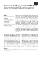
42.2.1 Bridge Foundation Types
From the perspective of SFSI, the foundation types commonly used for supporting bridge piers can
be classified in accordance with their soil-support configurations into four general types: (1) spread
footings, (2) caissons, (3) large-diameter shafts, and (4) slender-pile groups. These types as described
separately below are shown in Figure 42.1.

© 2000 by CRC Press LLC


FIGURE 42.1
pile group.

Bridge foundation types: (a) spread footing; (b) caisson; (c) large-diameter shafts; and (d) slender-

Spread Footings
Spread footings bearing directly on soil or rock are used to distribute the concentrated forces and
moments in bridge piers and/or abutments over sufficient areas to allow the underlying soil strata
to support such loads within allowable soil-bearing pressure limits. Of these loads, lateral forces are
resisted by a combination of friction on the foundation bottom surface and passive soil pressure
on its embedded vertical face. Spread footings are usually used on competent soils or rock which

© 2000 by CRC Press LLC


have high allowable bearing pressures. These foundations may be of several forms, such as (1)
isolated footings, each supporting a single column or wall pier; (2) combined footings, each supporting two or more closely spaced bridge columns; and (3) pedestals which are commonly used
for supporting steel bridge columns where it is desirable to terminate the structural steel above
grade for corrosion protection. Spread footings are generally designed to support the superimposed
forces and moments without uplifting or sliding. As such, inelastic action of the soils supporting
the footings is usually not significant.
Caissons
Caissons are large structural foundations, usually in water, that will permit dewatering to provide a dry
condition for excavation and construction of the bridge foundations. They can take many forms to suit
specific site conditions and can be constructed of reinforced concrete, steel, or composite steel and
concrete. Most caissons are in the form of a large cellular rectangular box or cylindrical shell structure

with a sealed base. They extend up from deep firm soil or rock-bearing strata to above mudline where
they support the bridge piers. The cellular spaces within the caissons are usually flooded and filled with
sand to some depth for greater stability. Caisson foundations are commonly used at deep-water sites
having deep soft soils. Transfer of the imposed forces and moments from a single pier takes place by
direct bearing of the caisson base on its supporting soil or rock stratum and by passive resistance of the
side soils over the embedded vertical face of the caisson. Since the soil-bearing area and the structural
rigidity of a caisson is very large, the transfer of forces from the caisson to the surrounding soil usually
involves negligible inelastic action at the soil–caisson interface.
Large-Diameter Shafts
These foundations consist of one or more large-diameter, usually in the range of 4 to 12 ft (1.2 to
3.6 m), reinforced concrete cast-in-drilled-hole (CIDH) or concrete cast-in-steel-shell (CISS) piles.
Such shafts are embedded in the soils to sufficient depths to reach firm soil strata or rock where a
high degree of fixity can be achieved, thus allowing the forces and moments imposed on the shafts
to be safely transferred to the embedment soils within allowable soil-bearing pressure limits and/or
allowable foundation displacement limits. The development of large-diameter drilling equipment
has made this type of foundation economically feasible; thus, its use has become increasingly
popular. In actual applications, the shafts often extend above ground surface or mudline to form a
single pier or a multiple-shaft pier foundation. Because of their larger expected lateral displacements
as compared with those of a large caisson, a moderate level of local soil nonlinearities is expected
to occur at the soil–shaft interfaces, especially near the ground surface or mudline. Such nonlinearities may have to be considered in design.
Slender-Pile Groups
Slender piles refer to those piles having a diameter or cross-sectional dimensions less than 2 ft (0.6 m).
These piles are usually installed in a group and provided with a rigid cap to form the foundation of a
bridge pier. Piles are used to extend the supporting foundations (pile caps) of a bridge down through
poor soils to more competent soil or rock. The resistance of a pile to a vertical load may be essentially
by point bearing when it is placed through very poor soils to a firm soil stratum or rock, or by friction
in case of piles that do not achieve point bearing. In real situations, the vertical resistance is usually
achieved by a combination of point bearing and side friction. Resistance to lateral loads is achieved by
a combination of soil passive pressure on the pile cap, soil resistance around the piles, and flexural
resistance of the piles. The uplift capacity of a pile is generally governed by the soil friction or cohesion

acting on the perimeter of the pile. Piles may be installed by driving or by casting in drilled holes. Driven
piles may be timber piles, concrete piles with or without prestress, steel piles in the form of pipe sections,
or steel piles in the form of structural shapes (e.g., H shape). Cast-in-drilled-hole piles are reinforced
concrete piles installed with or without steel casings. Because of their relatively small cross-sectional
dimensions, soil resistance to large pile loads usually develops large local soil nonlinearities that must

© 2000 by CRC Press LLC


be considered in design. Furthermore, since slender piles are normally installed in a group, mutual
interactions among piles will reduce overall group stiffness and capacity. The amounts of these reductions
depend on the pile-to-pile spacing and the degree ofsoil nonlinearity developed in resisting the loads.

42.2.2 Definition of SFSI Problem
For a bridge subjected to externally applied static and/or dynamic loadings on the aboveground
portion of the structure, the SFSI problem involves evaluation of the structural performance
(demand/capacity ratio) of the bridge under the applied loadings taking into account the effect of
SFI. Since in this case the ground has no initial motion prior to loading, the effect of SFI is to
provide the foundation–structure system with a flexible boundary condition at the soil–foundation
interface location when static loading is applied and a compliant boundary condition when dynamic
loading is applied. The SFI problem in this case therefore involves (1) evaluation of the soil–foundation interface boundary flexibility or compliance conditions for each bridge foundation, (2)
determination of the effects of these boundary conditions on the overall structural response of the
bridge (e.g., force, moment, or deformation) demands, and (3) evaluation of the resistance capacity
of each soil–foundation system that can be compared with the corresponding response demand in
assessing performance. That part of determining the soil–foundation interface boundary flexibilities
or compliances will be referred to subsequently in a gross term as the “foundation stiffness or
impedance problem”; that part of determining the structural response of the bridge as affected by
the soil–foundation boundary flexibilities or compliances will be referred to as the “foundation–structure interaction problem”; and that part of determining the resistance capacity of the
soil–foundation system will be referred to as the “foundation capacity problem.”
For a bridge structure subjected to seismic conditions, dynamic loadings are imposed on the

structure. These loadings, which originate with motions of the soil medium, are transmitted to the
structure through its foundations; therefore, the overall SFSI problem in this case involves, in
addition to the foundation impedance, FSI, and foundation capacity problems described above, the
evaluation of (1) the soil forces acting on the foundations as induced by the seismic ground motions,
referred to subsequently as the “seismic driving forces,” and (2) the effects of the free-field groundmotion-induced soil deformations on the soil–foundation boundary compliances and on the capacity of the soil–foundation systems. In order to evaluate the seismic driving forces on the foundations
and the effects of the free-field ground deformations on compliances and capacities of the soil–foundation systems, it is necessary to determine the variations of free-field motion within the ground
regions which interact with the foundations. This problem of determining the free-field ground
motion variations will be referred to herein as the “free-field site response problem.” As will be
shown later, the problem of evaluating the seismic driving forces on the foundations is equivalent
to determining the “effective or scattered foundation input motions” induced by the free-field soil
motions. This problem will be referred to here as the “foundation scattering problem.”
Thus, the overall SFSI problem for a bridge subjected to externally applied static and/or dynamic
loadings can be separated into the evaluation of (1) foundation stiffnesses or impedances, (2)
foundation–structure interactions, and (3) foundation capacities. For a bridge subjected to seismic
ground motion excitations, the SFSI problem involves two additional steps, namely, the evaluation
of free-field site response and foundation scattering. When solving the total SFSI problem, the effects
of the nonzero soil deformation state induced by the free-field seismic ground motions should be
evaluated in all five steps mentioned above.

42.2.3 Demand vs. Capacity Evaluations
As described previously, assessing the seismic performance of a bridge system requires evaluation
of SFSI involving two parts. One part is the evaluation of the effects of SFSI on the seismic-response
demands within the system; the other part is the evaluation of the seismic force and/or deformation

© 2000 by CRC Press LLC


capacities within the system. Ideally, a well-developed methodology should be one that is capable
of solving these two parts of the problem concurrently in one step using a unified suitable model
for the system. Unfortunately, to date, such a unified method has not yet been developed. Because

of the complexities of a real problem and the different emphases usually demanded of the solutions
for the two parts, different solution strategies and methods of analysis are warranted for solving
these two parts of the overall SFSI problem. To be more specific, evaluation on the demand side of
the problem is concerned with the overall SFSI system behavior which is controlled by the mass,
damping (energy dissipation), and stiffness properties, or, collectively, the impedance properties,
of the entire system; and, the solution must satisfy the dynamic equilibrium and compatibility
conditions of the global system. This system behavior is not sensitive, however, to approximations
made on local element behavior; thus, its evaluation does not require sophisticated characterizations
of the detailed constitutive relations of its local elements. For this reason, evaluation of demand has
often been carried out using a linear or equivalent linear analysis procedure. On the contrary,
evaluation of capacity must be concerned with the extreme behavior of local elements or subsystems;
therefore, it must place emphasis on the detailed constitutive behaviors of the local elements or
subsystems when deformed up to near-failure levels. Since only local behaviors are of concern, the
evaluation does not have to satisfy the global equilibrium and compatibility conditions of the system
fully. For this reason, evaluation of capacity is often obtained by conducting nonlinear analyses of
detailed local models of elements or subsystems or by testing of local members, connections, or
sub-assemblages, subjected to simple pseudo-static loading conditions.
Because of the distinct differences between effective demand and capacity analyses as described
above, the analysis procedures presented subsequently differentiate between these two parts of the
overall SFSI problem.

42.3 Current State-of-the-Practice
The evaluation of SFSI effects on bridges located in regions of high seismicity has not received as
much attention as for other critical engineered structures, such as dams, nuclear facilities, and
offshore structures. In the past, the evaluation of SFSI effects for bridges has, in most cases, been
regarded as a part of the bridge foundation design problem. As such, emphasis has been placed on
the evaluation of load-resisting capacities of various foundation systems with relatively little attention having been given to the evaluation of SFSI effects on seismic-response demands within the
complete bridge system. Only recently has formal SSI analysis methodologies and procedures,
developed and applied in other industries, been adopted and applied to seismic performance
evaluations of bridges [1], especially large important bridges [2,3].

Even though the SFSI problems for bridges pose their own distinct features (e.g., multiple
independent foundations of different types supported in highly variable soil conditions ranging
from hard to very soft), the current practice is to adopt, with minor modifications, the same
methodologies and procedures developed and practiced in other industries, most notably, the
nuclear power and offshore oil industries. Depending upon the foundation type and its soil-support
condition, the procedures currently being used in evaluating SFSI effects on bridges can broadly be
classified into two main methods, namely, the so-called elastodynamic method that has been
developed and practiced in the nuclear power industry for large foundations, and the so-called
empirical p–y method that has been developed and practiced in the offshore oil industry for pile
foundations. The bases and applicabilities of these two methods are described separately below.

42.3.1 Elastodynamic Method
This method is based on the well-established elastodynamic theory of wave propagation in a linear
elastic, viscoelastic, or constant-hysteresis-damped elastic half-space soil medium. The fundamental
element of this method is the constitutive relation between an applied harmonic point load and

© 2000 by CRC Press LLC


the corresponding dynamic response displacements within the medium called the dynamic Green’s
functions. Since these functions apply only to a linear elastic, visoelastic, or constant-hysteresisdamped elastic medium, they are valid only for linear SFSI problems. Since application of the
elastodynamic method of analysis uses only mass, stiffness, and damping properties of an SFSI
system, this method is suitable only for global system response analysis applications. However, by
adopting the same equivalent linearization procedure as that used in the seismic analysis of freefield soil response, e.g., that used in the computer program SHAKE [4], the method has been
extended to one that can accommodate global soil nonlinearities, i.e., those nonlinearities induced
in the free-field soil medium by the free-field seismic waves [5].
Application of the elastodynamic theory to dynamic SFSI started with the need for solving
machine–foundation vibration problems [6]. Along with other rapid advances in earthquake engineering in the 1970s, application of this theory was extended to solving seismic SSI problems for building
structures, especially those of nuclear power plants [7–9]. Such applications were enhanced by concurrent advances in analysis techniques for treating soil dynamics, including development of the complex
modulus representation of dynamic soil properties and use of the equivalent linearization technique

for treating ground-motion-induced soil nonlinearities [10–12]. These developments were further
enhanced by the extensive model calibration and methodology validation and refinement efforts carried
out in a comprehensive large-scale SSI field experimental program undertaken by the Electric Power
Research Institute (EPRI) in the 1980s [13]. All of these efforts contributed to advancing the elastodynamic method of SSI analysis currently being practiced in the nuclear power industry [5].
Because the elastodynamic method of analysis is capable of incorporating mass, stiffness, and
damping characteristics of each soil, foundation, and structure subsystem of the overall SFSI system,
it is capable of capturing the dynamic interactions between the soil and foundation subsystems and
between the foundations and structure subsystem; thus, it is suitable for seismic demand analyses.
However, since the method does not explicitly incorporate strength characteristics of the SFSI
system, it is not suitable for capacity evaluations.
As previously mentioned in Section 42.2.1, there are four types of foundation commonly used
for bridges: (1) spread footings, (2) caissons, (3) large-diameter shafts, and (4) slender-pile groups.
Since only small local soil nonlinearities are induced at the soil–foundation interfaces of spread
footings and caissons, application of the elastodynamic method of seismic demand analysis of the
complete SFSI system is valid. However, the validity of applying this method to large-diameter shaft
foundations depends on the diameter of the shafts and on the amplitude of the imposed loadings.
When the shaft diameter is large so that the load amplitudes produce only small local soil nonlinearities, the method is reasonably valid. However, when the shaft diameter is relatively small, the
larger-amplitude loadings will produce local soil nonlinearities sufficiently large to require that the
method be modified as discussed subsequently. Application of the elastodynamic method to slenderpile groups is usually invalid because of the large local soil nonlinearities which develop near the
pile boundaries. Only for very low amplitude loadings can the method be used for such foundations.

42.3.2 Empirical “p-y” Method
This method was originally developed for the evaluation of pile–foundation response due to lateral
loads [14–16] applied externally to offshore structures. As used, it characterizes the lateral soil
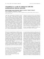
resistance per unit length of pile, p, as a function of the lateral displacement, y. The p–y relation is
generally developed on the basis of an empirical curve which reflects the nonlinear resistance of the
local soil surrounding the pile at a specified depth (Figure 42.2). Construction of the curve depends
mainly on soil material strength parameters, e.g., the friction angle, φ, for sands and cohesion, c,
for clays at the specified depth. For shallow soil depths where soil surface effects become important,
construction of these curves also depends on the local soil failure mechanisms, such as failure by a

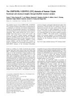
passive soil resistance wedge. Typical p–y curves developed for a pile at different soil depths are
shown in Figure 42.3. Once the set of p–y curves representing the soil resistances at discrete values

© 2000 by CRC Press LLC


FIGURE 42.2

Empirical p–y curves and secant modulus.

of depth along the length of the pile has been constructed, evaluation of pile response under a
specified set of lateral loads is accomplished by solving the problem of a beam supported laterally
on discrete nonlinear springs. The validity and applicability of this method are based on model
calibrations and correlations with field experimental results [15,16].
Based on the same model considerations used in developing the p–y curves for lateral response
analysis of piles, the method has been extended to treating the axial resistance of soils to piles per
unit length of pile, t, as a nonlinear function of the corresponding axial displacement, z, resulting
in the so-called axial t–z curve, and treating the axial resistance of the soils at the pile tip, Q, as a

© 2000 by CRC Press LLC


FIGURE 42.3

Typical p–y curves for a pile at different depths.

nonlinear function of the pile tip axial displacement, d, resulting in the so-called Q–d curve. Again,
the construction of the t–z and Q–d curves for a soil-supported pile is based on empirical curvilinear
forms and the soil strength parameters as functions of depth. By utilizing the set of p–y, t–z, and
Q–d curves developed for a pile foundation, the response of the pile subjected to general threedimensional (3-D) loadings applied at the pile head can be solved using the model of a 3-D beam

supported on discrete sets of nonlinear lateral p–y, axial t–z, and axial Q–d springs. The method as
described above for solving a soil-supported pile foundation subjected to applied loadings at the
pile head is referred to here as the empirical p–y method, even though it involves not just the lateral
p–y curves but also the axial t–z and Q–d curves for characterizing the soil resistances.
Since this method depends primarily on soil-resistance strength parameters and does not incorporate soil mass, stiffness, and damping characteristics, it is, strictly speaking, only applicable for
capacity evaluations of slender-pile foundations and is not suitable for seismic demand evaluations
because, as mentioned previously, a demand evaluation for an SFSI system requires the incorporation of the mass, stiffness, and damping properties of each of the constituent parts, namely, the
soil, foundation, and structure subsystems.
Even though the p–y method is not strictly suited to demand analyses, it is current practice in
performing seismic-demand evaluations for bridges supported on slender-pile group foundations
to make use of the empirical nonlinear p–y, t–z, and Q–d curves in developing a set of equivalent
linear lateral and axial soil springs attached to each pile at discrete elevations in the foundation.
The soil–pile systems developed in this manner are then coupled with the remaining bridge structure
to form the complete SFSI system for use in a seismic demand analysis. The initial stiffnesses of the
equivalent linear p–y, t–z, and Q–d soil springs are based on secant moduli of the nonlinear p–y,
t–y, and Q–d curves, respectively, at preselected levels of lateral and axial pile displacements, as
shown schematically in Figure 42.2. After completing the initial demand analysis, the amplitudes
of pile displacement are compared with the corresponding preselected amplitudes to check on their

© 2000 by CRC Press LLC


mutual compatibilities. If incompatibilities exist, the initial set of equivalent linear stiffnesses is
adjusted and a second demand analysis is performed. Such iterations continue until reasonable
compatibility is achieved. Since soil inertia and damping properties are not included in the abovedescribed demand analysis procedure, it must be considered approximate; however, it is reasonably
valid when the nonlinearities in the soil resistances become so large that the inelastic components
of soil deformations adjacent to piles are much larger than the corresponding elastic components.
This condition is true for a slender-pile group foundation subjected to relatively large amplitude
pile-head displacements. However, for a large-diameter shaft foundation, having larger soil-bearing
areas and higher shaft stiffnesses, the inelastic components of soil deformations may be of the same

order or even smaller than the elastic components, in which case, application of the empirical p–y
method for a demand analysis as described previously can result in substantial errors.

42.4 Seismic Inputs to SFSI System
The first step in conducting a seismic performance evaluation of a bridge structure is to define the
seismic input to the coupled soil–foundation–structure system. In a design situation, this input is
defined in terms of the expected free-field motions in the soil region surrounding each bridge
foundation. It is evident that to characterize such motions precisely is practically unachievable
within the present state of knowledge of seismic ground motions. Therefore, it is necessary to use
a rather simplistic approach in generating such motions for design purposes. The procedure most
commonly used for designing a large bridge is to (1) generate a three-component (two horizontal
and vertical) set of accelerograms representing the free-field ground motion at a “control point”
selected for the bridge site and (2) characterize the spatial variations of the free-field motions within
each soil region of interest relative to the control motions.
The control point is usually selected at the surface of bedrock (or surface of a firm soil stratum
in case of a deep soil site), referred to here as “rock outcrop,” at the location of a selected reference
pier; and the free-field seismic wave environment within the local soil region of each foundation is
assumed to be composed of vertically propagating plane shear (S) waves for the horizontal motions
and vertically propagating plane compression (P) waves for the vertical motions. For a bridge site
consisting of relatively soft topsoil deposits overlying competent soil strata or rock, the assumption
of vertically propagating plane waves over the depth of the foundations is reasonably valid as
confirmed by actual field downhole array recordings [17].
The design ground motion for a bridge is normally specified in terms of a set of parameter values
developed for the selected control point which include a set of target acceleration response spectra
(ARS) and a set of associated ground motion parameters for the design earthquake, namely (1)
magnitude, (2) source-to-site distance, (3) peak ground (rock-outcrop) acceleration (PGA), velocity
(PGV), and displacement (PGD), and (4) duration of strong shaking. For large important bridges,
these parameter values are usually established through regional seismic investigations coupled with
site-specific seismic hazard and ground motion studies, whereas, for small bridges, it is customary
to establish these values based on generic seismic study results such as contours of regional PGA

values and standard ARS curves for different general classes of site soil conditions.
For a long bridge supported on multiple piers which are in turn supported on multiple foundations spaced relatively far apart, the spatial variations of ground motions among the local soil regions
of the foundations need also be defined in the seismic input. Based on the results of analyses using
actual earthquake ground motion recordings obtained from strong motion instrument arrays, such
as the El Centro differential array in California and the SMART-1 array in Taiwan, the spatial
variations of free-field seismic motions have been characterized using two parameters: (1) apparent
horizontal wave propagation velocity (speed and direction) which controls the first-order spatial
variations of ground motion due to the seismic wave passage effect and (2) a set of horizontal and
vertical ground motion “coherency functions” which quantifies the second-order ground motion
variations due to scattering and complex 3-D wave propagation [18]. Thus, in addition to the design
© 2000 by CRC Press LLC


ground motion parameter values specified for the control motion, characterizing the design seismic
inputs to long bridges needs to include the two additional parameters mentioned above, namely,
(1) apparent horizontal wave velocity and (2) ground motion coherency functions; therefore, the
seismic input motions developed for the various pier foundation locations need to be compatible
with the values specified for these two additional parameters.
Having specified the design seismic ground motion parameters, the steps required in establishing
the pier foundation location-specific seismic input motions for a particular bridge are
1. Develop a three-component (two horizontal and vertical) set of free-field rock-outcrop
motion time histories which are compatible with the design target ARS and associated design
ground motion parameters applicable at a selected single control point location at the bridge
site (these motions are referred to here simply as the “response spectrum compatible time
histories” of control motion).
2. Generate response-spectrum-compatible time histories of free-field rock-outcrop motions at
each bridge pier support location such that their coherencies relative to the corresponding
components of the response spectrum compatible motions at the control point and at other
pier support locations are compatible with the wave passage parameters and the coherency
functions specified for the site (these motions are referred to here as “response spectrum and

coherency compatible motions).
3. Carry out free-field site response analyses for each pier support location to obtain the timehistories of free-field soil motions at specified discrete elevations over the full depth of each
foundation using the corresponding response spectrum and coherency compatible free-field
rock-outcrop motions as inputs.
In the following sections, procedures will be presented for generating the set of response spectrum
compatible rock-outcrop time histories of motion at the control point location and for generating
the sets of response spectrum and coherency compatible rock-outcrop time histories of motion at
all pier support locations, and guidelines will be given for performing free-field site response
analyses.

42.4.1 Free-Field Rock-Outcrop Motions at Control-Point Location
Given a prescribed set of target ARS and a set of associated design ground motion parameters for
a bridge site as described previously, the objective here is to develop a three-component set of time
histories of control motion that (1) provides a reasonable match to the corresponding target ARS
and (2) has time history characteristics reasonably compatible with the other specified associated
ground motion parameter values. In the past, several different procedures have been used for
developing rock-outcrop time histories of motion compatible with a prescribed set of target ARS.
These procedures are summarized as follows:
1. Response Spectrum Compatibility Time History Adjustment Method [19–22] — This method
as generally practiced starts by selecting a suitable three-component set of initial or “starting”
accelerograms and proceeds to adjust each of them iteratively, using either a time-domain
[21,23] or a frequency-domain [19,20,22] procedure, to achieve compatibility with the
specified target ARS and other associated parameter values. The time-domain adjustment
procedure usually produces only small local adjustments to the selected starting time histories,
thereby producing response spectrum compatible time histories closely resembling the initial
motions. The general “phasing” of the seismic waves in the starting time history is largely
maintained while achieving close compatibility with the target ARS: minor changes do occur,
however, in the phase relationships. The frequency-domain procedure as commonly used
retains the phase relationships of an initial motion, but does not always provide as close a fit
to the target spectrum as does the time-domain procedure. Also, the motion produced by

the frequency-domain procedure shows greater visual differences from the initial motion.
© 2000 by CRC Press LLC


2. Source-to-Site Numerical Model Time History Simulation Method [24–27] — This method
generally starts by constructing a numerical model to represent the controlling earthquake
source and source-to-site transmission and scattering functions, and then accelerograms are
synthesized for the site using numerical simulations based on various plausible fault-rupture
scenarios. Because of the large number of time history simulations required in order to achieve
a “stable” average ARS for the ensemble, this method is generally not practical for developing
a complete set of time histories to be used directly; rather it is generally used to supplement
a set of actual recorded accelerograms, in developing site-specific target response spectra and
associated ground motion parameter values.
3. Multiple Actual Recorded Time History Scaling Method [28,29] — This method starts by
selecting multiple 3-component sets (generally ≥7) of actual recorded accelerograms which
are subsequently scaled in such a way that the average of their response spectral ordinates
over the specified frequency (or period) range of interest matches the target ARS. Experience
in applying this method shows that its success depends very much on the selection of time
histories. Because of the lack of suitable recorded time histories, individual accelerograms
often have to be scaled up or down by large multiplication factors, thus raising questions
about the appropriateness of such scaling. Experience also indicates that unless a large ensemble of time histories (typically >20) are selected, it is generally difficult to achieve matching
of the target ARS over the entire spectral frequency (or period) range of interest.
4. Connecting Accelerogram Segments Method [55] — This method produces a synthetic time
history by connecting together segments of a number of actual recorded accelerograms in
such a way that the ARS of the resulting time history fits the target ARS reasonably well. It
generally requires producing a number of synthetic time histories to achieve acceptable
matching of the target spectrum over the entire frequency (or period) range of interest.
At the present time, Method 1 is considered most suitable and practical for bridge engineering
applications. In particular, the time-domain time history adjustment procedure which produces
only local time history disturbances has been applied widely in recent applications. This method

as developed by Lilhanand and Tseng [21] in 1988, which is based on earlier work by Kaul [30] in
1978, is described below.
The time-domain procedure for time history adjustment is based on the inherent definition of
a response spectrum and the recognition that the times of occurrence of the response spectral values
for the specified discrete frequencies and damping values are not significantly altered by adjustments
of the time history in the neighborhoods of these times. Thus, each adjustment, which is made by
adding a small perturbation, δa(t), to the selected initial or starting acceleration time history, a(t),
is carried out in an iterative manner such that, for each iteration, i, an adjusted acceleration time
history, ai(t), is obtained from the previous acceleration time history, a(i-1)(t), using the relation
a i(t) = a (i-1)(t) + δ a i(t)

(42.1)

The small local adjustment, δai(t), is determined by solving the integral equation
δRi(ωj, βk) =

∫

t jk

0

δai (τ)h jk(tjk – τ)d τ

(42.2)

which expresses the small change in the acceleration response value δRi(ωj, βk) for frequency ωj and
damping βk resulting from the local time history adjustment δai(t). This equation makes use of the
acceleration unit–impulse response function hjk(t) for a single-degree-of-freedom oscillator having
a natural frequency ωj and a damping ratio βk. Quantity tjk in the integral represents the time at

which its corresponding spectral value occurs, and τ is a time lag.

© 2000 by CRC Press LLC


By expressing δai(t) as a linear combination of impulse response functions with unknown coefficients, the above integral equation can be transformed into a system of linear algebraic equations
that can easily be solved for the unknown coefficients. Since the unit–impulse response functions
decay rapidly due to damping, they produce only localized perturbations on the acceleration time
history. By repeatedly applying the above adjustment, the desired degree of matching between the
response spectra of the modified motions and the corresponding target spectra is achieved, while,
in doing so, the general characteristics of the starting time history selected for adjustment are
preserved.
Since this method of time history modification produces only local disturbances to the starting
time history, the time history phasing characteristics (wave sequence or pattern) in the starting time
history are largely maintained. It is therefore important that the starting time history be selected
carefully. Each three-component set of starting accelerograms for a given bridge site should preferably be a set recorded during a past seismic event that has (1) a source mechanism similar to that
of the controlling design earthquake, (2) a magnitude within about ±0.5 of the target controlling
earthquake magnitude, and (3) a closest source-to-site distance within 10 km of the target sourceto-site distance. The selected recorded accelerograms should have their PGA, PGV, and PGD values
and their strong shaking durations within a range of ±25% of the target values specified for the
bridge site and they should represent free-field surface recordings on rock, rocklike, or a stiff soil
site; no recordings on a soft site should be used. For a close-in controlling seismic event, e.g., within
about 10 km of the site, the selected accelerograms should contain a definite velocity pulse or the
so-called fling. When such recordings are not available, Method 2 described previously can be used
to generate a starting set of time histories having an appropriate fling or to modify the starting set
of recorded motions to include the desired directional velocity pulse.
Having selected a three-component set of starting time histories, the horizontal components
should be transformed into their principal components and the corresponding principal directions
should be evaluated [31]. These principal components should then be made response spectrum
compatible using the time-domain adjustment procedure described above or the standard frequency-domain adjustment procedure[20,22,32]. Using the lat er procedure, only the Fourier
t

amplitude spectrum, not the phase spectrum, is adjusted iteratively.
The target acceleration response spectra are in general identical for the two horizontal principal
components of motion; however, a distinct target spectrum is specified for the vertical component.
In such cases, the adjusted response spectrum compatible horizontal components can be oriented
horizontally along any two orthogonal coordinate axes in the horizontal plane considered suitable
for structural analysis applications. However, for bridge projects that have controlling seismic
events with close-in seismic sources, the two horizontal target response spectra representing
motions along a specified set of orthogonal axes are somewhat different, especially in the lowfrequency (long-period) range; thus, the response spectrum compatible time histories must have
the same definitive orientation. In this case, the generated three-component set of response
spectrum compatible time histories should be used in conjunction with their orientation. The
application of this three-component set of motions in a different coordinate orientation requires
transforming the motions to the new coordinate system. It should be noted that such a transformation of the components will generally result in time histories that are not fully compatible
with the original target response spectra. Thus, if response spectrum compatibility is desired in
a specific coordinate orientation (such as in the longitudinal and transverse directions of the
bridge), target response spectra in the specific orientation should be generated first and then a
three-component set of fully response spectrum compatible time histories should be generated
for this specific coordinate system.
As an example, a three-component set of response spectrum compatible time histories of control
motion, generated using the time-domain time history adjustment procedure, is shown in
Figure 42.4.

© 2000 by CRC Press LLC


FIGURE 42.4

Examples of a three-component set of response spectrum compatible time histories of control motion.

© 2000 by CRC Press LLC

42.4.2 Free-Field Rock-Outcrop Motions at Bridge Pier Support Locations
As mentioned previously, characterization of the spatial variations of ground motions for engineering purposes is based on a set of wave passage parameters and ground motion coherency functions.
The wave passage parameters currently used are the apparent horizontal seismic wave speed, V, and
its direction angle θ relative to an axis normal to the longitudinal axis of the bridge. Studies of
strong- and weak-motion array data including those in California, Taiwan, and Japan show that the
apparent horizontal speed of S-waves in the direction of propagation is typically in the 2 to 3 km/s
range [18,33]. In applications, the apparent wave-velocity vector showing speed and direction must
be projected along the bridge axis giving the apparent wave speed in that direction as expressed by
Vbridge =

V
sin θ

(42.3)

To be realistic, when θ becomes small, a minimum angle for θ, say, 30°, should be used in order to
account for waves arriving in directions different from the specified direction.
The spatial coherency of the free-field components of motion in a single direction at various
locations on the ground surface has been parameterized by a complex coherency function defined
by the relation
Γ ij(iω) =

Sij (iω )
Sii (ω ) S jj (ω )

i, j = 1, 2, …, n locations

(42.4)

in which Sij(iω) is the smoothed complex cross-power spectral density function and Sii(ω) and Sjj(ω)
are the smoothed real power spectral density (PSD) functions of the components of motion at
locations i and j. The notation iω in the above equation is used to indicate that the coefficients
Sij(iω) are complex valued (contain both real and imaginary parts) and are dependent upon excitation frequency ω. Based on analyses of strong-motion array data, a set of generic coherency
functions for the horizontal and vertical ground motions has been developed [34]. These functions
for discrete separation distances between locations i and j are plotted against frequency in
Figure 42.5.
Given a three-component set of response spectrum compatible time histories of rock-outcrop
motions developed for the selected control point location and a specified set of wave passage
parameters and “target” coherency functions as described above, response spectrum compatible and
coherency compatible multiple-support rock-outcrop motions applicable to each pier support location of the bridge can be generated using the procedure presented below. This procedure is based
on the “marching method” developed by Hao et al. [32] in 1989 and extended by Tseng et al. [35]
in 1993.
Neglecting, for the time being, ground motion attenuation along the bridge axis, the components
of rock-outcrop motions at all pier support locations in a specific direction have PSD functions
which are common with the PSD function So(ω) specified for the control motion, i.e.,
S ii(ω) = S jj(ω) = So(ω) = u o(iω) 2

(42.5)

where uo(iω) is the Fourier transform of the corresponding component of control motion, uo(t).
By substituting Eq. (42.5) into Eq. (42.4), one obtains
S ij(iω) = Γ ij(iω) So(ω)

© 2000 by CRC Press LLC

(42.6)


FIGURE 42.5

Example of coherency functions of frequency at discrete separation distances.

which can be rewritten in a matrix form for all pier support locations as follows:
S(iω) = Γ (iω) So(ω)

(42.7)

Since, by definition, the coherency matrix Γ (iω) is an Hermitian matrix, it can be decomposed
into a complex conjugate pair of lower and upper triangular matrices L(iω) and L * (iω )T as
expressed by

Γ (iω) = L(iω) L * (iω )T
© 2000 by CRC Press LLC

(42.8)


in which the symbol * denotes complex conjugate. In proceeding, let
u(iω) = L(iω) ηφi (iω ) uo (iω )

(42.9)

in which u(ω) is a vector containing components of motion ui(ω) for locations, i = 1, 2, …, n; and,
ηφi (iω ) = {eiφi ( ω )} is a vector containing unit amplitude components having random-phase angles
φi(ω). If φi(ω) and φj(ω) are uniformly distributed random-phase angles, the relations
E[ ηφi (iω ) η* j (iω )] = 0
φ

if i ≠ j

E[ ηφi (iω ) η* j (iω )] = 1
φ

if i = j

(42.10)

will be satisfied, where the symbol E[ ] represents ensemble average. It can easily be shown that
the ensemble of motions generated using Eq. (42.9) will satisfy Eq. (42.7). Thus, if the rock-outcrop
motions at all pier support locations are generated from the corresponding motions at the control
point location using Eq. (42.9), the resulting motions at all locations will satisfy, on an ensemble
basis, the coherency functions specified for the site. Since the matrix L(iω) in Eq. (42.9) is a lower
triangular matrix having its diagonal elements equal to unity, the generation of coherency compatible motions at all pier locations can be achieved by marching from one pier location to the next
in a sequential manner starting with the control pier location.
In generating the coherency compatible motions using Eq. (42.9), the phase angle shifts at various
pier locations due to the single plane-wave passage at the constant speed Vbridge defined by Eq. (42.3)
can be incorporated into the term ηφ (iω ) . Since the motions at the control point location are
i
response spectrum compatible, the coherency compatible motions generated at all other pier locations using the above-described procedure will be approximately response spectrum compatible.
However, an improvement on their response spectrum compatibility is generally required, which
can be done by adjusting their Fourier amplitudes but keeping their Fourier phase angles unchanged.
By keeping these angles unchanged, the coherencies among the adjusted motions are not affected.
Consequently, the adjusted motions will not only be response spectrum compatible, but will also
be coherency compatible.
In generating the response spectrum- and coherency-compatible motions at all pier locations by
the procedure described above, the ground motion attenuation effect has been ignored. For a long
bridge located close to the controlling seismic source, attenuation of motion with distance away
from the control pier location should be considered. This can be achieved by scaling the generated
motions at various pier locations by appropriate scaling factors determined from an appropriate

ground motion attenuation relation. The acceleration time histories generated for all pier locations
should be integrated to obtain their corresponding velocity and displacement time histories, which
should be checked to ensure against having numerically generated baseline drifts. Relative displacement time histories between the control pier location and successive pier locations should also be
checked to ensure that they are reasonable. The rock-outcrop motions finally obtained should then
be used in appropriate site-response analyses to develop the corresponding free-field soil motions
required in conducting the SFSI analyses for each pier location.

42.4.3 Free-Field Soil Motions
As previously mentioned, the seismic inputs to large bridges are defined in terms of the expected
free-field soil motions at discrete elevations over the entire depth of each foundation. Such motions
must be evaluated through location-specific site-response analyses using the corresponding previously described rock-outcrop free-field motions as inputs to appropriately defined soil–bedrock

© 2000 by CRC Press LLC


models. Usually, as mentioned previously, these models are based on the assumption that the
horizontal and vertical free-field soil motions are produced by upward/downward propagation of
one-dimensional shear and compression waves, respectively, as caused by the upward propagation
of incident waves in the underlying rock or firm soil formation. Consistent with these types of
motion, it is assumed that the local soil medium surrounding each foundation consists of uniform
horizontal layers of infinite lateral extent. Wave reflections and refractions will occur at all interfaces
of adjacent layers, including the soil–bedrock interface, and reflections of the waves will occur at
the soil surface. Computer program SHAKE [4,44] is most commonly used to carry out the abovedescribed one-dimensional type of site-response analysis. For a long bridge having a widely varying
soil profile from end to end, such site-response analyses must be repeated for different soil columns
representative of the changing profile.
The cyclic free-field soil deformations produced at a particular bridge site by a maximum expected
earthquake are usually of the nonlinear hysteretic form. Since the SHAKE computer program treats
a linear system, the soil column being analyzed must be modeled in an equivalent linearized manner.
To obtain the equivalent linearized form, the soil parameters in the model are modified after each
consecutive linear time history response analysis is complete, which continues until convergence to

strain-compatible parameters are reached.
For generating horizontal free-field motions produced by vertically propagating shear waves, the
needed equivalent linear soil parameters are the shear modulus G and the hysteretic damping ratio
β. These parameters, as prepared by Vucetic and Dobry [36] in 1991 for clay and by Sun et al. [37]
in 1988 and by the Electric Power Research Institute (EPRI) for sand, are plotted in Figures 42.6
and 42.7, respectively, as functions of shear strain γ. The shear modulus is plotted in its nondimensional form G/Gmax where Gmax is the in situ shear modulus at very low strains (γ ≤ 10–4%). The
shear modulus G must be obtained from cyclic shear tests, while Gmax can be obtained using Gmax =
ρVs2 in which ρ is mass density of the soil and Vs is the in situ shear wave velocity obtained by field
measurement. If shear wave velocities are not available, Gmax can be estimated using published
empirical formulas which correlate shear wave velocity or shear modulus with blow counts and/or
other soil parameters [38–43]. To obtain the equivalent linearized values of G/Gmax and β following
each consecutive time history response analysis, values are taken from the G/Gmax vs. γ and β vs. γ
relations at the effective shear strain level defined as γeff = αγmax in which γmax is the maximum shear
strain reached in the last analysis and α is the effective strain factor. In the past, α has usually been
assigned the value 0.65; however, other values have been proposed (e.g., Idriss and Sun [44]). The
equivalent linear time history response analyses are performed in an iterative manner, with soil
parameter adjustments being made after each analysis, until the effective shear strain converges to
essentially the same value used in the previous iteration [45]. This normally takes four to eight
iterations to reach 90 to 95% of full convergence when the effective shear strains do not exceed 1
to 2%. When the maximum strain exceeds 2%, a nonlinear site-response analysis is more appropriate. Computer programs available for this purpose are DESRA [46], DYNAFLOW [47], DYNAID
[48], and SUMDES [49].
For generating vertical free-field motions produced by vertically propagating compression waves,
the needed soil parameters are the low-strain constrained elastic modulus Ep = ρVp2 , where Vp is
the compression wave velocity, and the corresponding damping ratio. The variations of these soil
parameters with compressive strain have not as yet been well established. At the present time, vertical
site-response analyses have generally been carried out using the low-strain constrained elastic
moduli, Ep, directly and the strain-compatible damping ratios obtained from the horizontal response
analyses, but limited to a maximum value of 10%, without any further strain-compatibility iterations. For soils submerged in water, the value of Ep should not be less than the compression wave
velocity of water.
Having generated acceleration free-field time histories of motion using the SHAKE computer

program, the corresponding velocity and displacement time histories should be obtained through

© 2000 by CRC Press LLC


FIGURE 42.6 Equivalent linear shear modulus and hysteretic damping ratio as functions of shear strain for clay.
(Source: Vucetic, M. and Dobry, R., J. Geotech. Eng. ASCE, 117(1), 89-107, 1991. With permission.)

single and double integrations of the acceleration time histories. Should unrealistic drifts appear in
the displacement time histories, appropriate corrections should be applied. Should such drifts
appear in a straight-line fashion, it usually indicates that the durations specified for Fourier transforming the recorded accelerograms are too short; thus, increasing these durations will usually
correct the problem. If the baseline drifts depart significantly from a simple straight line, this tends
to indicate that the analysis results may be unreliable; in which case, they should be carefully checked
before being used. Time histories of free-field relative displacement between pairs of pier locations
should also be generated and then be checked to judge the reasonableness of the results obtained.

© 2000 by CRC Press LLC


FIGURE 42.7 Equivalent linear shear modulus and hysteretic damping ratio as functions of shear strain for sand.
(Source: Sun, J. I. et al., Reort No. UBC/EERC-88/15, Earthquake Engineer Research Center, University of California,
Berkeley, 1988.)

42.5 Characterization of Soil–Foundation System
The core of the dynamic SFSI problem for a bridge is the interaction between its structure–foundation system and the supporting soil medium, which, for analysis purposes, can be considered to
be a full half-space. The fundamental step in solving this problem is to characterize the constitutive
relations between the dynamic forces acting on each foundation of the bridge at its interface
boundary with the soil and the corresponding foundation motions, expressed in terms of the
displacements, velocities, and accelerations. Such forces are here called the soil–foundation interaction forces. For a bridge subjected to externally applied loadings, such as dead, live, wind, and
© 2000 by CRC Press LLC

wave loadings, these SFI forces are functions of the foundation motions only; however, for a bridge
subjected to seismic loadings, they are functions of the free-field soil motions as well.
Let h be the total number of degrees of freedom (DOF) of the bridge foundations as defined at
˙˙
˙
their soil–foundation interface boundaries; uh(t), uh (t ) , and uh (t ) be the corresponding foundation
˙
˙˙
displacement, velocity, and acceleration vectors, respectively; and uh (t ) , uh (t ) , and uh (t ) be the
free-field soil displacement, velocity, and acceleration vectors in the h DOF, respectively; and let
fh(t) be the corresponding SFI force vector. By using these notations, characterization of the SFI
forces under seismic conditions can be expressed in the general vectorial functional form:
˙
˙˙
˙
˙˙
fh(t) = ℑh (uh(t), uh (t ) , uh (t ) , uh (t ) uh (t ) , uh (t ) )

(42.11)

Since the soils in the local region immediately surrounding each foundation may behave nonlinearly
under imposed foundation loadings, the form of ℑh is, in general, a nonlinear function of displacements uh(t) and uh (t ) and their corresponding velocities and accelerations.
For a capacity evaluation, the nonlinear form of ℑh should be retained and used directly for
determining the SFI forces as functions of the foundation and soil displacements. Evaluation of this
form should be based on a suitable nonlinear model for the soil medium coupled with appropriate
boundary conditions, subjected to imposed loadings which are usually much simplified compared
with the actual induced loadings. This part of the evaluation will be discussed further in Section 42.8.
For a demand evaluation, the nonlinear form of ℑh is often linearized and then transformed to

˙
˙˙
˙˙
˙
the frequency domain. Letting uh(iω), uh (iω ) , uh (iω ) , uh (iω ) , uh (iω ) , uh (iω ) , and fh(iω) be the
˙ (t ) , u (t ) , and fh(t), respectively, and making
˙˙
˙˙
˙
Fourier transforms of uh(t), uh (t ) , uh (t ) , uh (t ) , uh
h
use of the relations
˙
uh (iω ) = iω uh (iω ) ;

˙˙
uh (iω ) = −ω 2 uh (iω )

˙
uh (iω ) = iω uh (iω ) ;

˙˙
uh (iω ) = −ω 2 uh (iω ) ,

and
(42.12)

Equation (42.11) can be cast into the more convenient form:
fh(iω) = ℑ h ( uh (iω ), uh (iω ) )

(42.13)

To characterize the linear functional form of ℑh, it is necessary to solve the dynamic boundaryvalue problem for a half-space soil medium subjected to force boundary conditions prescribed at
the soil–foundation interfaces. This problem is referred to here as the “soil impedance” problem,
which is a part of the foundation impedance problem referred to earlier in Section 42.2.2.
In linearized form, Eq. (42.13) can be expressed as
fh(iω) = Ghh(iω) {uh (iω ) − uh (iω )}

(42.14)

in which fh(iω) represents the force vector acting on the soil medium by the foundation and the
matrix Ghh(iω) is a complex, frequency-dependent coefficient matrix called here the “soil impedance
matrix.”
Define a force vector fh (iω ) by the relation
fh (iω ) = Ghh(iω) uh (iω )

© 2000 by CRC Press LLC

(42.15)


This force vector represents the internal dynamic forces acting on the bridge foundations at their
soil–foundation interface boundaries resulting from the free-field soil motions when the foundations are held fixed, i.e., uh (iω ) = 0. The force vector fh (iω ) as defined in Eq. (42.15) is the “seismic
driving force” vector mentioned previously in Section 42.2.2. Depending upon the type of bridge
foundation, the characterization of the soil impedance matrix Ghh(iω) and associated free-field soil
input motion vector uh (iω ) for demand analysis purposes may be established utilizing different
soil models as described below.

42.5.1 Elastodynamic Model
As mentioned in Section 42.3.1, for a large bridge foundation such as a large spread footing, caisson,

or single or multiple shafts having very large diameters, for which the nonlinearities occurring in
the local soil region immediately adjacent to the foundation are small, the soil impedance matrix
Ghh(iω) can be evaluated utilizing the dynamic Green’s functions (dynamic displacements of the
soil medium due to harmonic point-load excitations) obtained from the solution of a dynamic
boundary-value problem of a linear damped-elastic half-space soil medium subjected to harmonic
point loads applied at each of the h DOF on the soil–foundation interface boundaries. Such solutions
have been obtained in analytical form for a linear damped-elastic continuum half-space soil medium
by Apsel [50] in 1979. Because of complexities in the analytical solution, dynamic Green’s functions
have only been obtained for foundations having relatively simple soil–foundation interface geometries, e.g., rectangular, cylindrical, or spherical soil–foundation interface geometries, supported in
simple soil media. In practical applications, the dynamic Green’s functions are often obtained in
numerical forms based on a finite-element discretization of the half-space soil medium and a
corresponding discretization of the soil–foundation interface boundaries using a computer program
such as SASSI [51], which has the capability of properly simulating the wave radiation boundary
conditions at the far field of the half-space soil medium. The use of finite-element soil models to
evaluate the dynamic Green’s functions in numerical form has the advantage that foundations having
arbitrary soil–foundation interface geometries can be easily handled; it, however, suffers from the
disadvantage that the highest frequency, i.e., cutoff frequency, of motion for which a reliable solution
can be obtained is limited by size of the finite element used for modeling the soil medium.
Having evaluated the dynamic Green’s functions using the procedure described above, the desired
soil impedance matrix can then be obtained by inverting, frequency-by-frequency, the “soil compliance
matrix,” which is the matrix of Green’s function values evaluated for each specified frequency ω. Because
the dynamic Green’s functions are complex valued and frequency dependent, the coefficients of the
resulting soil impedance matrix are also complex-valued and frequency dependent. The real parts of
the soil impedance coefficients represent the dynamic stiffnesses of the soil medium which also incorporate the soil inertia effects; the imaginary parts of the coefficients represent the energy losses resulting
from both soil material damping and radiation of stress waves into the far-field soil medium. Thus, the
soil impedance matrix as developed reflects the overall dynamic characteristics of the soil medium as
related to the motion of the foundation at the soil–foundation interfaces.
Because of the presence of the foundation excavation cavities in the soil medium, the vector of freefield soil motions uh (iω ) prescribed at the soil–foundation interface boundaries has to be derived from
the seismic input motions of the free-field soil medium without the foundation excavation cavities as
described in Section 42.4. The derivation of the motion vector uh (iω ) requires the solution of a dynamic

boundary-value problem for the free-field half-space soil medium having foundation excavation cavities
subjected to a specified seismic wave input such that the resulting solution satisfies the traction-free
conditions at the surfaces of the foundation excavation cavities. Thus, the resulting seismic response
motions, uh (iω ) , reflect the effects of seismic wave scattering due to the presence of the cavities. These
motions are, therefore, referred to here as the “scattered free-field soil input motions.”
The effects of seismic wave scattering depend on the relative relation between the characteristic
dimension, l f , of the foundation and the specific seismic input wave length, λ, of interest, where

© 2000 by CRC Press LLC


λ = 2πVs/ω or 2πVp/ω for vertically propagating plane shear or compression waves, respectively; Vs
and Vp are, as defined previously, the shear and compression wave velocities of the soil medium,
respectively. If the input seismic wave length λ is much longer than the characteristic length l f ,
the effect of wave scattering will be negligible; on the other hand, when λ ≤ l f , the effect of wave
scattering will be significant. Since the wave length λ is a function of the frequency of input motion,
the effect of wave scattering is also frequency dependent. Thus, it is evident that the effect of wave
scattering is much more important for a large bridge foundation, such as a large caisson or a group
of very large diameter shafts, than for a small foundation having a small characteristic dimension,
such as a slender-pile group; it can also be readily deduced that the scattering effect is more
significant for foundations supported in soft soil sites than for those in stiff soil sites.
The characterization of the soil impedance matrix utilizing an elastodynamic model of the soil
medium as described above requires soil material characterization constants which include (1) mass
density, ρ; (2) shear and constrained elastic moduli, G and Ep (or shear and compression wave
velocities, Vs and Vp); and (3) constant-hysteresis damping ratio, β. As discussed previously in
Section 42.4.3, the soil shear modulus decreases while the soil hysteresis damping ratio increases as
functions of soil shear strains induced in the free-field soil medium due to the seismic input motions.
The effects of these so-called global soil nonlinearities can be easily incorporated into the soil
impedance matrix based on an elastodynamic model by using the free-field-motion-induced straincompatible soil shear moduli and damping ratios as the soil material constants in the evaluation of
the dynamic Green’s functions. For convenience of later discussions, the soil impedance matrix,

e
Ghh(iω), characterized using an elastodynamic model will be denoted by the symbol Ghh (iω ) .

42.5.2 Empirical p–y Model
As discussed in Section 42.3.2, for a slender-pile group foundation for which soil nonlinearities
occurring in the local soil regions immediately adjacent to the piles dominate the behavior of the
foundation under loadings, the characterization of the soil resistances to pile deflections has often
relied on empirically derived p–y curves for lateral resistance and t–z and Q–d curves for axial
resistance. For such a foundation, the characterization of the soil impedance matrix needed for
demand analysis purposes can be made by using the secant moduli derived from the nonlinear p–y,
t–z, and Q–d curves, as indicated schematically in Figure 42.2. Since the development of these
empirical curves has been based upon static or pseudo-static test results, it does not incorporate
the soil inertia and material damping effects. Thus, the resulting soil impedance matrix developed
from the secant moduli of the p–y, t–z, and Q–d curves reflects only the static soil stiffnesses but
not the soil inertia and soil material damping characteristics. Hence, the soil impedance matrix so
obtained is a real-valued constant coefficient matrix applicable at the zero frequency (ω = 0); it,
however, is a function of the foundation displacement amplitude. This matrix is designated here as
s
e
Ghh (0) to differentiate it from the soil impedance matrix Ghh (iω ) defined previously. Thus,
Eq. (42.14) in this case is given by
s
fh(iω) = Ghh (0) {uh (iω ) − uh (iω )}

(42.16)

s
where Ghh (0) depends on the amplitudes of the relative displacement vector ∆uh(iω) defined by

∆uh(iω) = uh (iω ) − uh (iω )

(42.17)

As mentioned previously in Section 42.3.2, the construction of the p–y, t–z, and Q–d curves depends
only on the strength parameters but not on the stiffness parameters of the soil medium; thus, the
effects of global soil nonlinearities on the dynamic stiffnesses of the soil medium, as caused by soil
shear modulus decrease and soil-damping increase as functions of free-field-motion-induced soil

© 2000 by CRC Press LLC


shear strains, cannot be incorporated into the soil impedance matrix developed from these curves.
Furthermore, since these curves are developed on the basis of results from field tests in which there
are no free-field ground-motion-induced soil deformations, the effects of such global soil nonlinearities on the soil strength characterization parameters and hence the p–y, t–z, and Q–d curves
cannot be incorporated.
Because of the small cross-sectional dimensions of slender piles, the seismic wave-scattering effect
due to the presence of pile cavities is usually negligible; thus, the scattered free-field soil input
motions uh (iω ) in this case are often taken to be the same as the free-field soil motions when the
cavities are not present.

42.5.3 Hybrid Model
From the discussions in the above two sections, it is clear that characterization of the SFI forces for
demand analysis purposes can be achieved using either an elastodynamic model or an empirical
p–y model for the soil medium, each of which has its own merits and deficiencies. The elastodynamic
model is capable of incorporating soil inertia, damping (material and radiation), and stiffness
characteristics, and it can incorporate the effects of global soil nonlinearities induced by the freefield soil motions in an equivalent linearized manner. However, it suffers from the deficiency that
it does not allow for easy incorporation of the effects of local soil nonlinearities. On the contrary,
the empirical p–y model can properly capture the effects of local soil nonlinearities in an equivalent
linearized form; however, it suffers from the deficiencies of not being able to simulate soil inertia
and damping effects properly, and it cannot treat the effects of global soil nonlinearities. Since the

capabilities of the two models are mutually complementary, it is logical to combine the elastodynamic model with the empirical p–y model in a series form such that the combined model has the
desired capabilities of both models. This combined model is referred to here as the “hybrid model.”
To develop the hybrid model, let the relative displacement vector, ∆uh(iω), between the foundation
displacement vector uh(iω) and the scattered free-field soil input displacement vector uh (iω ) , as
defined by Eq. (42.17), be decomposed into a component representing the relative displacements
at the soil–foundation interface boundary resulting from the elastic deformation of the global soil
medium outside of the soil–foundation interface, designated as ∆uhe(iω), and a component representing the relative displacements at the same boundary resulting from the inelastic deformations
of the local soil regions adjacent the foundation, designated as ∆uhi(iω); thus,
∆uh(iω) = ∆uhi(iω) + ∆uhe(iω)

(42.18)

Let fhe (iω) represent the elastic force vector which can be characterized in terms of the elastic
e
relative displacement vector uh (iω) using the elastodynamic model, in which case
e
e
fhe(iω) = Ghh (iω ) ∆uh (iω )

(42.19)

where Ghhe(iω) is the soil impedance matrix as defined previously in Section 42.5.1, which can be
evaluated using an elastodynamic model. Let fhi(iω) represent the inelastic force vector which is
assumed to be related to ∆uhi(iω) by the relation
i
i
fhi(iω) = Ghh (iω ) ∆uh (iω )

(42.20)

i
The characterization of the matrix Ghh (iω ) can be accomplished by utilizing the soil secant
s
stiffness matrix G hh ( 0 ) developed from the empirical p–y model by the procedure discussed below.
e
i
Solving Eqs. (42.19) and (42.20) for ∆uh (iω ) and ∆uh (iω ) , respectively, substituting these
relative displacement vectors into Eq. (42.18), and making use of the force continuity condition

© 2000 by CRC Press LLC